
| 일 | 월 | 화 | 수 | 목 | 금 | 토 |
|---|---|---|---|---|---|---|
| 1 | 2 | 3 | 4 | 5 | ||
| 6 | 7 | 8 | 9 | 10 | 11 | 12 |
| 13 | 14 | 15 | 16 | 17 | 18 | 19 |
| 20 | 21 | 22 | 23 | 24 | 25 | 26 |
| 27 | 28 | 29 | 30 |
- 공공빅데이터청년인재양성
- 머신러닝
- 텍스트마이닝
- SQL
- 분석변수처리
- Kaggle
- 오버샘플링
- DL
- 공빅데
- 데이터전처리
- 클러스터링
- Keras
- 2023공공빅데이터청년인재양성
- machinelearning
- 공빅
- 2023공빅데
- ADSP
- data
- ADsP3과목
- 데이터분석
- 2023공공빅데이터청년인재양성후기
- textmining
- NLP
- ML
- DeepLearning
- 빅데이터
- k-means
- 공공빅데이터청년인턴
- datascience
- decisiontree
- Today
- Total
愛林
[Python/MachineLearning] 앙상블 알고리즘 (Ensemble Algorithms) : 랜덤 포레스트 (Random Forest) 본문
[Python/MachineLearning] 앙상블 알고리즘 (Ensemble Algorithms) : 랜덤 포레스트 (Random Forest)
愛林 2022. 8. 23. 01:37
랜덤 포레스트 (Random Forest)
랜덤 포레스트란, 여러 개의 결정 트리를 임의적으로 학습하는 방식의 앙상블 방법이다.
Bagging 보다 더 많은 임의성을 주어서 학습기를 생성한 후,
이를 선형 결합하여 최종 학습기를 만드는 방법이다. (분류/회귀가 있다.)
Bagging 처럼 데이터를 반복 복원추출을 진행할 뿐만 아니라,
거기에 더해서 변수 또한 random 하게 추출해서 다양한 모델을 만든다.
배깅 기법을 통해서 임의 복원추출되는 훈련용 데이터를 생성 후, 각각의 트리를 생성한다.
뽑을 변수의 개수는 분석가가 직접 선택해야 하는 하이퍼 파라미터이다.
예측 결과를 투표, 평균, 확률 등으로 종합해서 예측 결과를 도출해내는 모델이다.
의사결정나무가 하나의 큰 나무였다면,
랜덤포레스트는 하나의 큰 숲이라고 생각하면 된다!
의사결정나무가 앙상블된 것이 랜덤포레스트이다.
렌덤포레스트는 우리가 이전에 배웠던 배깅 (Bagging) 방법을 쓴다.
https://wndofla123.tistory.com/67
[Python/MachineLearning] 앙상블 알고리즘 (Ensemble Algorithms) : 배깅 (Bagging)
이전에는 의사결정나무에 대해 알아보았다. 이번엔 앙상블 알고리즘에 대해 알아보자. 앙상블 알고리즘 (Ensemble Algorithms) 앙상블 알고리즘이란, 일련의 분류 기준을 구성한 후 예측 가중치 투표
wndofla123.tistory.com
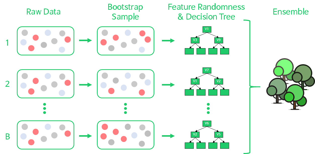
Rawdata 에서 Bootstrap Sample 을 추출해내고,
이를 통해서 의사결정나무를 만든다. 배깅을 사용하기 때문에, 비복원 추출을 하고 중복을 허용한다.
이후에는이러한 의사결정나무 모델을 앙상블시켜 랜덤포레스트 모델을 생성한다.
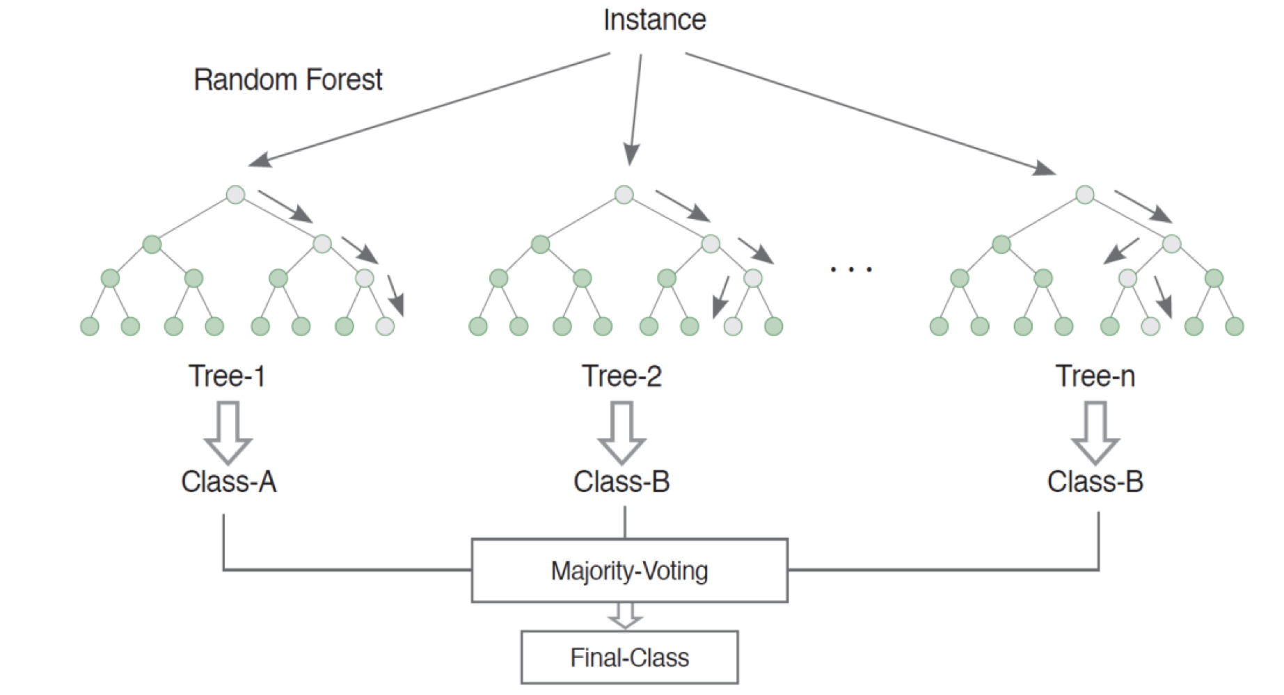
모든 예측기들이 훈련을 마치면, 앙상블은 모든 예측기들을 모아서 결과를 투표한다.
랜덤포레스트는 회귀와 분류가 있는데, 분류에서는 통계적 최빈값을 사용하고,
회귀에서는 평균을 계산하게 된다.
의사결정나무 개개인은 원본 훈련 세트로 훈련시킨것보다 훨씬 편향되어 있으나,
수집함수를 통과하게 되면 편향과 분산이 모두 감소하게 된다.
일반적으로 앙상블의 결과를 원본 데이터셋으로 하나의 예측기를 훈련시킬 때보다
편향은 비슷하나 분산은 줄어든다.
Bagging RandomForest 실습
sklearn의 MakeMoon 을 사용하여 실습해보자.
from sklearn.datasets import make_moons
import seaborn as sns
# 데이터 생성
X, y = make_moons(n_samples=500, noise=0.30, random_state=42)
# 산점도
sns.scatterplot(X[:,0],X[:,1], y)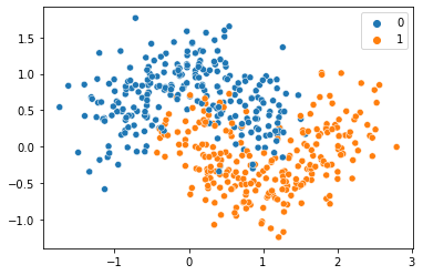
데이터가 잘 생성이 되었다.
from sklearn.ensemble import BaggingClassifier
from sklearn.tree import DecisionTreeClassifier
from sklearn.metrics import accuracy_score
from sklearn.model_selection import train_test_split

# 학습 / 검증 분할
X_train, X_test, y_train, y_test = train_test_split(X, y, random_state=42)

# 모델생성
tree_clf = DecisionTreeClassifier(random_state=42)
tree_clf.fit(X_train, y_train)
y_pred_tree = tree_clf.predict(X_test)

bag_clf = BaggingClassifier(
    DecisionTreeClassifier(), n_estimators=500,
    max_samples=100, bootstrap=True, random_state=42)
bag_clf.fit(X_train, y_train)
y_pred = bag_clf.predict(X_test)
Bagging, DecisionTree 라이브러리들을 import 해주고,
정확도 검증을 위해 accuracy_socre 와 테스트 데이터 학습 데이터 분류를 위한 train_test_split 까지 불러와주었다.
이후 데이터들을 분할하고, 데이터들을 학습시켜준 다음 모델을 생성해준다.
from sklearn.metrics import accuracy_score
print("배깅 accuracy :",accuracy_score(y_test, y_pred))
배깅 accuracy : 0.904
tree_clf = DecisionTreeClassifier(random_state=42)
tree_clf.fit(X_train, y_train)
y_pred_tree = tree_clf.predict(X_test)
print("의사결정나무 accuracy :", accuracy_score(y_test, y_pred_tree))
의사결정나무 accuracy : 0.856
각각의 정확도를 살펴보았다.
이제 시각화를 통해서 분류를 얼마나 잘 해냈는 지 확인해보자.
from matplotlib.colors import ListedColormap
import matplotlib.pyplot as plt
import numpy as np

def plot_decision_boundary(clf, X, y, axes=[-1.5, 2.45, -1, 1.5], alpha=0.5, contour=True):
    x1s = np.linspace(axes[0], axes[1], 100)
    x2s = np.linspace(axes[2], axes[3], 100)
    x1, x2 = np.meshgrid(x1s, x2s)
    X_new = np.c_[x1.ravel(), x2.ravel()]
    y_pred = clf.predict(X_new).reshape(x1.shape)
    custom_cmap = ListedColormap(['#FFD8D8','#9898ff','#B2EBF4'])
    plt.contourf(x1, x2, y_pred, #alpha=0.3,
                 cmap=custom_cmap)
    if contour:
        custom_cmap2 = ListedColormap(['#7d7d58','#4c4c7f','#507d50'])
        plt.contour(x1, x2, y_pred, #alpha=0.8,
                    cmap=custom_cmap2)
    plt.plot(X[:, 0][y==0], X[:, 1][y==0], "ro", alpha=alpha)
    plt.plot(X[:, 0][y==1], X[:, 1][y==1], "bs", alpha=alpha)
    plt.axis(axes)
    plt.xlabel(r"$x_1$", fontsize=18)
    plt.ylabel(r"$x_2$", fontsize=18, rotation=0)
시각화시켜주는 함수를 만들었다.
fig, axes = plt.subplots(ncols=2, figsize=(12,6), sharey=True)
plt.sca(axes[0])
plot_decision_boundary(tree_clf, X, y)
plt.title("Decision Tree", fontsize=18)
plt.sca(axes[1])
plot_decision_boundary(bag_clf, X, y)
plt.title("Decision Trees with Bagging", fontsize=18)
plt.ylabel("")
plt.show()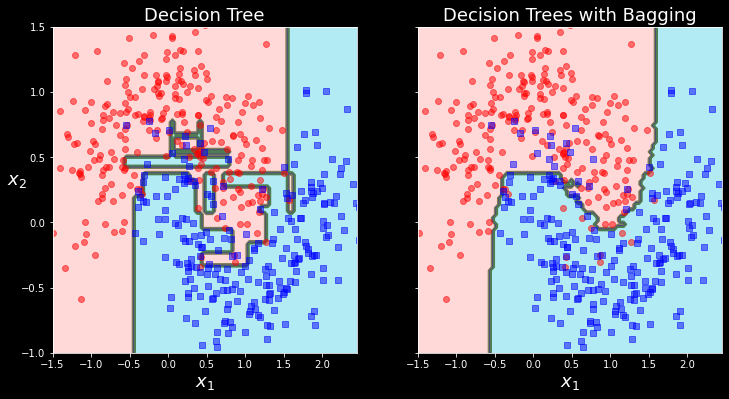
랜덤포레스트는 배깅방법을 적용한 의사결정나무의 숲이다.
전형적으로 max sample 을 train set 의 크기로 지정한다.
Bagging Classifier 에 Decision Tree Classifier 을 넣어 만드는 대신에,
결정 트리에 최적화 되어있어 사용하기 편하게 RandomForestClassifier 을 사용할 수 있다.
굳이 위에서 한 것처럼 Bagging 분류기 안에 Decision Tree 를 하지 않아도 된다는 말이다.
회귀를 위한 RandomForestRegressor 도 있다.
다음은 최대 16개의 leaf node 를 갖는 500개 트리로 이루어진 RandomForestClassifier 을 여러
CPU 코어에서 훈련시키는 코드이다.
from sklearn.ensemble import RandomForestClassifier

rnd_clf = RandomForestClassifier(n_estimators=500, max_leaf_nodes=16, random_state=42)
rnd_clf.fit(X_train, y_train)

y_pred_rf = rnd_clf.predict(X_test)
RandomForestClassifier 는 몇 가지 예외가 있으나, DecisionTreeClassifier 의 파라미터와
앙상블 자체를 제어하는 데 필요한 BaggingClassifier 의 파라미터를 모두 갖고 있다.
랜덤 포레스트 알고리즘은 트리의 노드를 분할할 때, 전체 특성 중에서 최선의 특성을 찾는 대신
무작위로 선택한 특성 후보 중에서 최적의 특성을 찾는 식으로 무작위성을 더 주입한다.
이는 결국 트리를 더욱 다양하게 만들고 편향을 손해보는 대신 분산을 낮추어서 전체적으로 보았을 때
더 훌륭한 모델을 만들어낸다.
그럼, RandomForestClassifier 와 BaggingClassifier 내부에 DecisionTree로 랜덤포레스트 분류기와
유사하게 만든 모델로 비교해보자. (위에서 만든 BaggingClassifier 내부의 DecisionTree)
from sklearn.ensemble import RandomForestClassifier

rnd_clf = RandomForestClassifier(n_estimators=500, max_leaf_nodes=16, random_state=42)
rnd_clf.fit(X_train, y_train)

y_pred_rf = rnd_clf.predict(X_test)

bag_clf.fit(X_train, y_train)
y_pred = bag_clf.predict(X_test)

np.sum(y_pred == y_pred_rf) / len(y_pred)0.976거의 1로 유사하게 나왔다.
fig, axes = plt.subplots(ncols=2, figsize=(20,10), sharey=True)
plt.sca(axes[0])
plot_decision_boundary(rnd_clf, X, y)
plt.title("Random Forest", fontsize=18)
plt.sca(axes[1])
plot_decision_boundary(bag_clf, X, y)
plt.title("Decision Trees with Bagging", fontsize=18)
plt.ylabel("")
plt.show()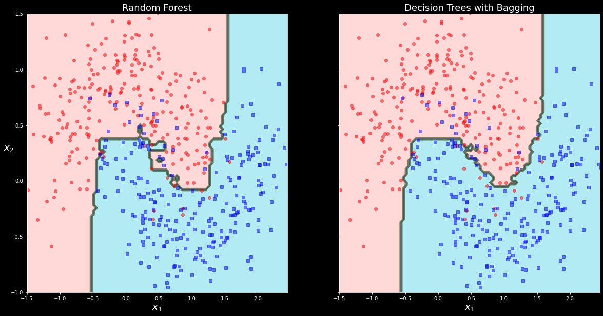
시각화했을때도 거의 유사하게 분류가 된 것을 볼 수 있으나,
RandomForest 모델이 쪼오끔 더 좋은 결과를 보여주고 있는 것 같다.
RandomForest 변수 중요도 시각화
RandomForest 의 또 다른 장점은 특성의 상대적 중요도를 측정하기 쉽다는 것이다.
Sklearn 은 어떤 특성을 사용한 노드가 평균적으로 불순도를 얼마나 감소시키는 지 확인하여
특성의 중요도를 측정한다.
Skelarn 은 훈련이 끝난 뒤 특성마다 자동으로 이 점수를 계산하고 전체 합이 1이 되도록
결과값을 정규화시키는데, 이 값은 feature_importances 변수에 저장되어 있다.
iris 데이터셋에 RandomForestClassifier 을 훈련시키고, 각 특성의 중요도를 출력하여 시각화해보자.
from sklearn.datasets import load_iris
iris = load_iris()

# X, y 할당
X = iris["data"]
y = iris['target']

# Train, Test 분할
from sklearn.model_selection import train_test_split
X_train, X_test, y_train, y_test = train_test_split(X, y, stratify=y, random_state=42)
_state=42)
rnd_clf.fit(X_train, y_train)
rnd_clf_pred = rnd_clf.predict(X_test) #X_test 예측
rnd_clf_acc = rnd_clf.score(X_test, y_test ) # 정확도(Accuracy) 출력
#----------------------------------------------
print("랜덤포레스트 training accuracy :", rnd_clf.score( X_train, y_train )*100, "%")
print("랜덤포레스트 test accuracy :", rnd_clf_acc * 100, "%")
#----------------------------------------------
print("--------------------------------------------------------------------------")
print(classification_report(y_test, rnd_clf_pred))
print("--------------------------------------------------------------------------")
print(confusion_matrix(y_test, rnd_clf_pred))
print("--------------------------------------------------------------------------")
#----------------------------------------------
end = time.time()
print('Execution time is:')
print(end - start)
plot_confusion_matrix(rnd_clf, X_test, y_test , cmap='YlGn')
plt.title("<< Random Forest >>")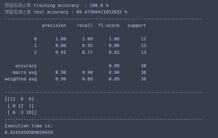
랜덤포레스트 모델의 정확도는 89% 정도가 나왔다.
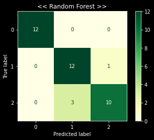
대체적으로 잘 수행하고 있는 모델인 것 같다.
이제 특성 중요도를 살펴보고, 시각화해보자.
# 특성 중요도 출력
for name, score in zip(iris["feature_names"], rnd_clf.feature_importances_):
    print([name, score])

# 특성 중요도 시각화
sns.barplot(x=rnd_clf.feature_importances_, y=iris.feature_names)
plt.title("Random forest_feature importance")# 특성 중요도 출력
for name, score in zip(iris["feature_names"], rnd_clf.feature_importances_):
    print([name, score])

# 특성 중요도 시각화
sns.barplot(x=rnd_clf.feature_importances_, y=iris.feature_names)
plt.title("Random forest_feature importance")
['sepal length (cm)', 0.1219238899824993]
['sepal width (cm)', 0.028212457341966667]
['petal length (cm)', 0.44200866611709616]
['petal width (cm)', 0.40785498655843794]
['sepal length (cm)', 0.1219238899824993]
['sepal width (cm)', 0.028212457341966667]
['petal length (cm)', 0.44200866611709616]
['petal width (cm)', 0.40785498655843794]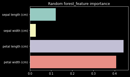
Petal Length 꽃잎의 길이가 가장 중요도가 높고,
Petal Width 꽃잎의 넓이가 그 다음으로 중요도가 높은 것을 알 수 있었다.
'Data Science > Machine Learning' 카테고리의 다른 글
| [Python/ML] 분류 알고리즘 (Classification Algorithm) : 나이브 베이즈 (Naive Bayes) (2) | 2022.08.31 |
|---|---|
| [Python/ML] 앙상블 알고리즘 (Ensemble Algorithms) : 부스팅 (Boosting) (3) | 2022.08.26 |
| [Python/MachineLearning] 앙상블 알고리즘 (Ensemble Algorithms) : 보팅 (Votting) (2) | 2022.08.22 |
| [Python/MachineLearning] 앙상블 알고리즘 (Ensemble Algorithms) : 배깅 (Bagging) (2) | 2022.08.21 |
| [Python/ML] Mini Project - Water Quality Data (2) | 2022.08.17 |


