[Text Mining] 텍스트 마이닝 - Gensim 을 이용한 토픽 모델링 (Topic Modeling) , LDA

저번 시간에는 Scikit Learn 을 이용하여 LDA 토픽 모델링을 진행해보았다.

오늘은 Gensim 이라는 패키지를 이용하여 토픽 모델링을 진행해보자.

 

https://radimrehurek.com/gensim/models/word2vec.html

Gensim: topic modelling for humans

---

GENSIM

 

Gensim 은 Word2Vec 으로 잘 알려져 있으며,

토픽 모델링을 비롯해서 의미적인 자연어 처리를 위한 다양한 라이브러리를 제공한다.

사이킷런과는 달리 토큰화 도구를 따로 제공하지 않는다.

그래서 텍스트 전처리를 따로 한 다음, 텍스트 전처리 결과를 넘겨주어야 한다.

 

 

Dictionary 

전처리를 위한 주요 클래스이다.

특성집합을 Dictionary 라고 한다.

토큰과 gensim 내부 id 를 매칭하는 사전이다.

 

- filter_extremes() : keep_n (max_features 와 유사), no_below (min_df 와 유사),

no_above (max_df) 와 유사 를 이용하여 필터링을 하고 사전(특성집합)을 생성한다.

 

- doc2bow() : 각 토큰화 결과를 특성 벡터(bow) 로 변환한다.

CounterVectorizer 와 유사하다.

 

 

---

GENSIM을 이용한 토픽 모델링 실습

 

NLTK 의 RegexpTokenizer 를 이용하여 토큰화를 진행해보자.

불용어 처리를 하고, 3자 이상의 단어만 사용한다.

 

이전에 했던 newsgroup_data 를 이용하여 실습할 것이다.

 

!pip install gensim
!pip install pyldavis

gensim 과 시각화를 위한 pylavis 를 설치해주어야 한다.

 

from nltk.corpus import stopwords
from nltk.tokenize import RegexpTokenizer
cachedStopWords = stopwords.words("english")
RegTok = RegexpTokenizer("[\w']{3,}") # 정규포현식으로 토크나이저를 정의
english_stops = set(stopwords.words('english')) # 영어 불용어를 가져옴
def tokenizer(text):
    tokens = RegTok.tokenize(text.lower())
    # stopwords 제외
    words = [word for word in tokens if (word not in english_stops) and len(word) > 2] 
    return words
texts = [tokenizer(news) for news in newsgroups_train.data]

토큰화 결과를 texts 에 저장했다.

from gensim.corpora.dictionary import Dictionary
# 토큰화 결과로부터 dictionay 생성
dictionary = Dictionary(texts)
print('#Number of initial unique words in documents:', len(dictionary))
# 문서 빈도수가 너무 적거나 높은 단어를 필터링하고 특성을 단어의 빈도 순으로 선택
dictionary.filter_extremes(keep_n = 2000, no_below=5, no_above=0.5)
print('#Number of unique words after removing rare and common words:', len(dictionary))
# 카운트 벡터로 변환
corpus = [dictionary.doc2bow(text) for text in texts] 
print('#Number of unique tokens: %d' % len(dictionary)) 
print('#Number of documents: %d' % len(corpus))

Dictionary 를 불러오고,

토큰화 결과로 dictionary 를 생성하해준다.

최대 2000개의 단어를 사용하고 이전에 했던 것처럼 5번 이하 사용된 글자는 사용하지 않고,

50% 이상으로 사용된 글자도 사용하지 않는다.

#Number of initial unique words in documents: 46466
#Number of unique words after removing rare and common words: 2000
#Number of unique tokens: 2000
#Number of documents: 3219

Gensim 에서는 CountVector 를 corpus 라고 칭한다. (이전에는 말뭉치를 corpus라고 칭했음)

45466개이다.

위에서 생략하기로 한 단어들을 생략하고 거른 뒤 2000개의 단얼르 사용했다.

2000개의 tokens 를 사용했고,

문서는 3219개이다. 

 

 

gensim의 gensim.models.LdaModel 을 사용하여 LDA 를 진행해보자.

 

gensim.models.LdaModel

 

- corpus : 변환된 특성 벡터, 즉 dictionary.doc2bow() 의 실행 결과

 

- id2word : 참조할 특성 집합, 생성한 Dictionary 객체

 

- passes : 알고리즘 반복 횟수

 

- num_topics : 토픽의수

 

- print_topics(num_words) : 토픽의 단어 분포를 상위 num_words 수만큼  출력한다.

이전에 sklearn 을 사용했을때는 따로 함수로 만들어주었어야 했다.

 

Sklearn 과는 달리 LdaModel 로 객체를 생성하면서 바로 토픽 모델링이 실행된다.

앞서 생성한 corpus 와 dictionary 를 corpus , id2word 의 인수로 전달해준다.

최대 반복횟수와 토픽의 수를 지정해주고,

토픽의단어분포를보고 싶을 땐 print_topics 를 사용한다.

 

 

from gensim.models import LdaModel
num_topics = 9
passes = 5
model = LdaModel(corpus=corpus, id2word=dictionary,\
                       passes=passes, num_topics=num_topics, \
                       random_state=7)

토픽의 개수는 이전과 동일한 9개,

최대 반복횟수는 5번으로 제한한다.

corpus (카운트벡터)를 corpus 에 넣어주고,

위에서 생성한 Dictionary 를 id2word 에 넣어준다.

알고리즘 반복횟수는 5번, 토픽 개수 9개, random_state 또한 설정해준다.

 

model.print_topics(num_words=10)

[(0,
  '0.015*"com" + 0.015*"would" + 0.014*"keith" + 0.013*"caltech" + 0.012*"article" + 0.011*"sgi" + 0.011*"nntp" + 0.010*"posting" + 0.010*"host" + 0.009*"system"'),
 (1,
  '0.014*"objective" + 0.013*"com" + 0.013*"article" + 0.012*"uiuc" + 0.012*"say" + 0.012*"morality" + 0.012*"one" + 0.010*"frank" + 0.010*"faq" + 0.009*"values"'),
 (2,
  '0.027*"com" + 0.026*"posting" + 0.026*"host" + 0.026*"nntp" + 0.023*"access" + 0.015*"digex" + 0.014*"article" + 0.013*"university" + 0.012*"pat" + 0.012*"cwru"'),
 (3,
  '0.031*"space" + 0.017*"nasa" + 0.009*"gov" + 0.007*"orbit" + 0.006*"research" + 0.006*"university" + 0.006*"earth" + 0.006*"information" + 0.005*"data" + 0.005*"center"'),
 (4,
  '0.025*"com" + 0.012*"article" + 0.012*"ibm" + 0.011*"would" + 0.010*"henry" + 0.009*"toronto" + 0.009*"one" + 0.009*"like" + 0.009*"get" + 0.008*"work"'),
 (5,
  '0.022*"key" + 0.014*"encryption" + 0.013*"clipper" + 0.012*"chip" + 0.011*"com" + 0.009*"government" + 0.009*"would" + 0.008*"keys" + 0.008*"use" + 0.007*"security"'),
 (6,
  '0.020*"scsi" + 0.019*"drive" + 0.013*"com" + 0.011*"card" + 0.010*"ide" + 0.009*"one" + 0.009*"controller" + 0.008*"bus" + 0.008*"disk" + 0.007*"system"'),
 (7,
  '0.016*"graphics" + 0.011*"image" + 0.009*"ftp" + 0.009*"file" + 0.009*"files" + 0.009*"com" + 0.008*"use" + 0.008*"available" + 0.008*"mail" + 0.007*"program"'),
 (8,
  '0.013*"god" + 0.012*"one" + 0.012*"people" + 0.010*"would" + 0.008*"com" + 0.007*"think" + 0.007*"jesus" + 0.006*"even" + 0.006*"say" + 0.006*"article"')]

토픽의 비중과 단어를 함께 출력해준다.

용이하지만 한 눈에 알아보기는 어렵다.

 

print("#topic distribution of the first document: ", model.get_document_topics(corpus)
[0])

#topic distribution of the first document:  [(0, 0.6954689), (8, 0.30036935)]

첫 번째 문서의 토픽 분류이다.

첫 번째 토픽의 70% 정도, 9번째 토픽이 30% 정도를 차지한다.

 

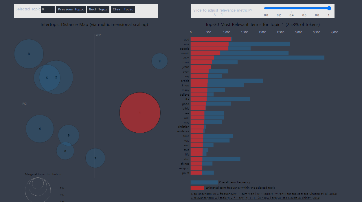
pyLDAvis 를 사용하면 위의 결과를 쉽게 시각화 할 수 있다.

 

import pyLDAvis
import pyLDAvis.gensim_models as gensimvis
pyLDAvis.enable_notebook()
# LDA 모형을 pyLDAvis 객체에 전달
lda_viz = gensimvis.prepare(model, corpus, dictionary)
lda_viz

jupyter notebook 환경에서 작업했기에,

notebook 에서 사용가능하도록 만들어주었다.

이후 위의 LDA 모형을 pyLDAvis 에 전달해주고, corpus 와 dictionary 를 넣어주었다.

 

상당히 신기하게 시각화가 진행된다.

 

 

 

 

 ※ 해당 자료는 모두 공공 빅데이터 청년 인턴 교육자료들을 참고합니다.