
| 일 | 월 | 화 | 수 | 목 | 금 | 토 |
|---|---|---|---|---|---|---|
| 1 | 2 | 3 | ||||
| 4 | 5 | 6 | 7 | 8 | 9 | 10 |
| 11 | 12 | 13 | 14 | 15 | 16 | 17 |
| 18 | 19 | 20 | 21 | 22 | 23 | 24 |
| 25 | 26 | 27 | 28 | 29 | 30 | 31 |
- decisiontree
- 빅데이터
- data
- SQL
- 2023공빅데
- 공빅
- DL
- k-means
- 공공빅데이터청년인턴
- 클러스터링
- DeepLearning
- 분석변수처리
- 2023공공빅데이터청년인재양성후기
- Kaggle
- 공공빅데이터청년인재양성
- 데이터전처리
- 오버샘플링
- datascience
- 머신러닝
- 텍스트마이닝
- textmining
- NLP
- Keras
- 데이터분석
- ADsP3과목
- 공빅데
- ML
- 2023공공빅데이터청년인재양성
- machinelearning
- ADSP
- Today
- Total
愛林
[Python/ML] Mini Project - Water Quality Data 본문
Mini Project - Water Quality Data

Water Quality Data 를 이용하여 미니 프로젝트를 진행해보자.
kaggle 의 Water Quality Data 를 이용했다.
https://www.kaggle.com/datasets/adityakadiwal/water-potability
Water Quality
Drinking water potability
www.kaggle.com
[ 안전한 식수에 대한 접근은 기본적인 인권이자 건강 보호를 위한 효과적인 정책의 구성 요소인 건강에 필수적이다.
이것은 국가, 지역 및 지역 수준에서 보건 및 개발 문제로 중요합니다.
일부 지역에서는 의료 역효과와 의료 비용의 감소가 개입 비용을 능가하기 때문에 상수도와 위생에 대한 투자가
순 경제적 이익을 창출할 수 있는 것으로 나타났다. ]
해당 데이터는 pH값(pH), Hardness(경도), Solids(고형물), Chloramins(클로라민), Sulfate(황산염), Conductivity(전도도), Organic_Carbon(유기탄소), Trihalomethanes(트리할로메탄), Turbidity(탁도), Potability(이식성)
에 관한 정보가 포함되어있다.
먼저, 라이브러리를 불러와주자.
# 기본 라이브러리
import numpy as np
import pandas as pd

# 시각화 라이브러리
import matplotlib.pyplot as plt
import seaborn as sns
import plotly
import plotly.express as px
import plotly.graph_objs as go
from pywaffle import Waffle

# 데이터 전처리 라이브러리
from sklearn.preprocessing import StandardScaler,MinMaxScaler
from sklearn.model_selection import train_test_split

# 모델링 라이브러리
from sklearn.linear_model import LogisticRegression
from sklearn.svm import SVC , LinearSVC
from sklearn.neighbors import KNeighborsClassifier
from sklearn.tree import DecisionTreeClassifier
from sklearn.ensemble import RandomForestClassifier , AdaBoostClassifier , GradientBoostingClassifier
from sklearn.naive_bayes import GaussianNB , BernoulliNB
from lightgbm import LGBMClassifier

# 모델 평가 및 파라미터 튜닝 라이브러리
from sklearn.metrics import precision_score,accuracy_score, classification_report, plot_confusion_matrix, confusion_matrix
from sklearn.model_selection import GridSearchCV
나는 lightgbm 과 pywaffle 이라는 라이브러리가 없어서 설치해주었다.
lightgbm 은 부스팅 계열 알고리즘에서 각광받는 모델이라고 알려져있다. Boosting 관련인듯.
pywaffle 은 구글링하니까 안 나오는데 차트를 만드는 라이브러리인 것 같다 .
# 데이터 불러오기
df = pd.read_csv('./water_potability.csv')
df
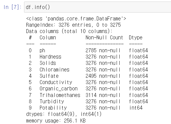
3280개 정보의 빅데이터 ...
df.isnull().sum()ph 491
Hardness 0
Solids 0
Chloramines 0
Sulfate 781
Conductivity 0
Organic_carbon 0
Trihalomethanes 162
Turbidity 0
Potability 0
dtype: int64Ph, 황산염, 트리할로메탄에서 결측치가 꽤나 보인다.
# axis=0 : 결측값이 있는 행 제거
# axis=1 : 결측값이 있는 열 제거
df = df.dropna(axis=0)
dropna() 를 사용해서 결측값이 있는 행을 제거해주었다. axis = 0이 행 삭제이다.

데이터가 많이 날아가긴 했지만 ?
아무튼 간에 2011 개의 null 값이 없는 데이터들이 남았다.
우리의 최종 목표는 설명 변수 9개로 반응변수 Potability 를 분류하는 것이다.
Potability 는 이식성으로 사람이 물을 먹어도 안전한지 여부를 나타낸다.
여기서 1은 음용가능함을 의미하고 0은 음용불가함을 의미한다.
EDA (탐색적 데이터 분석)
탐색적 데이터분석 EDA 를 진행해보자.
Waffle 을 이용해서 수질의 0, 1(식수) 비율이 어떤 지 알아보았다.
from pywaffle import Waffle
Potability = df['Potability'].value_counts()
plt.style.use('dark_background')

fig = plt.figure(
    FigureClass = Waffle,
    rows = 4,
    columns = 4,
    values = Potability,
    labels = ['{} - {}'.format(a, b) for a, b in zip(Potability.index, Potability)],
    legend = {
        'loc': 'upper left',
        'bbox_to_anchor': (1, 1),
        'fontsize': 20,
        'labelcolor': 'linecolor',
        'title': 'Water Quality',
        'title_fontsize': 20,
        },
    font_size = 60,
    icon_legend = True,
    figsize = (10, 8),
)

plt.title('Water Quality Distribution', fontsize = 20)
plt.show()
못 먹는 물이 훨씬 많다 1200 개의 데이터가 못 먹는 물이다.
811 개의 데이터가 식수이다.
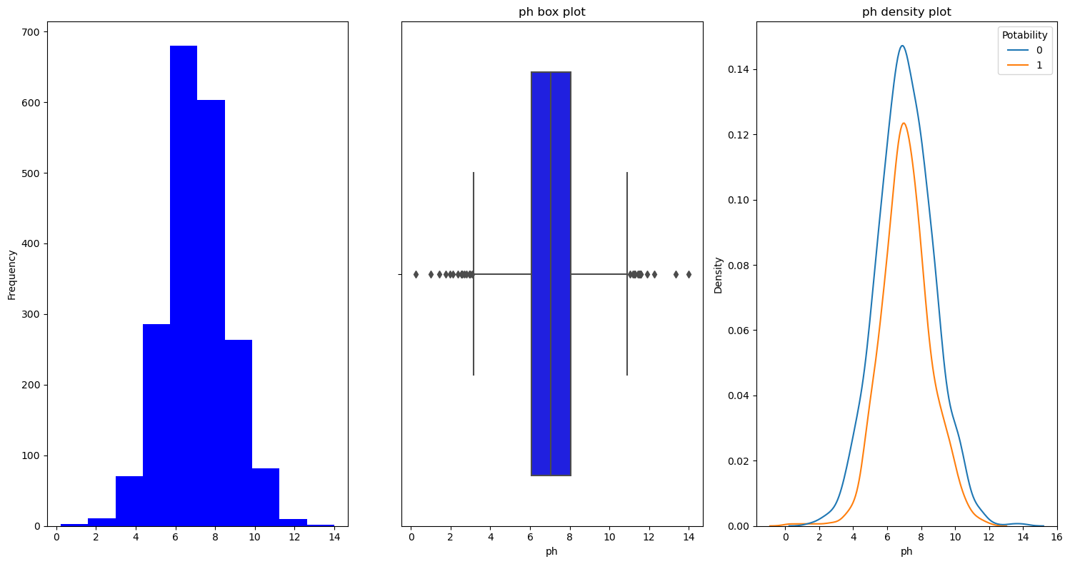
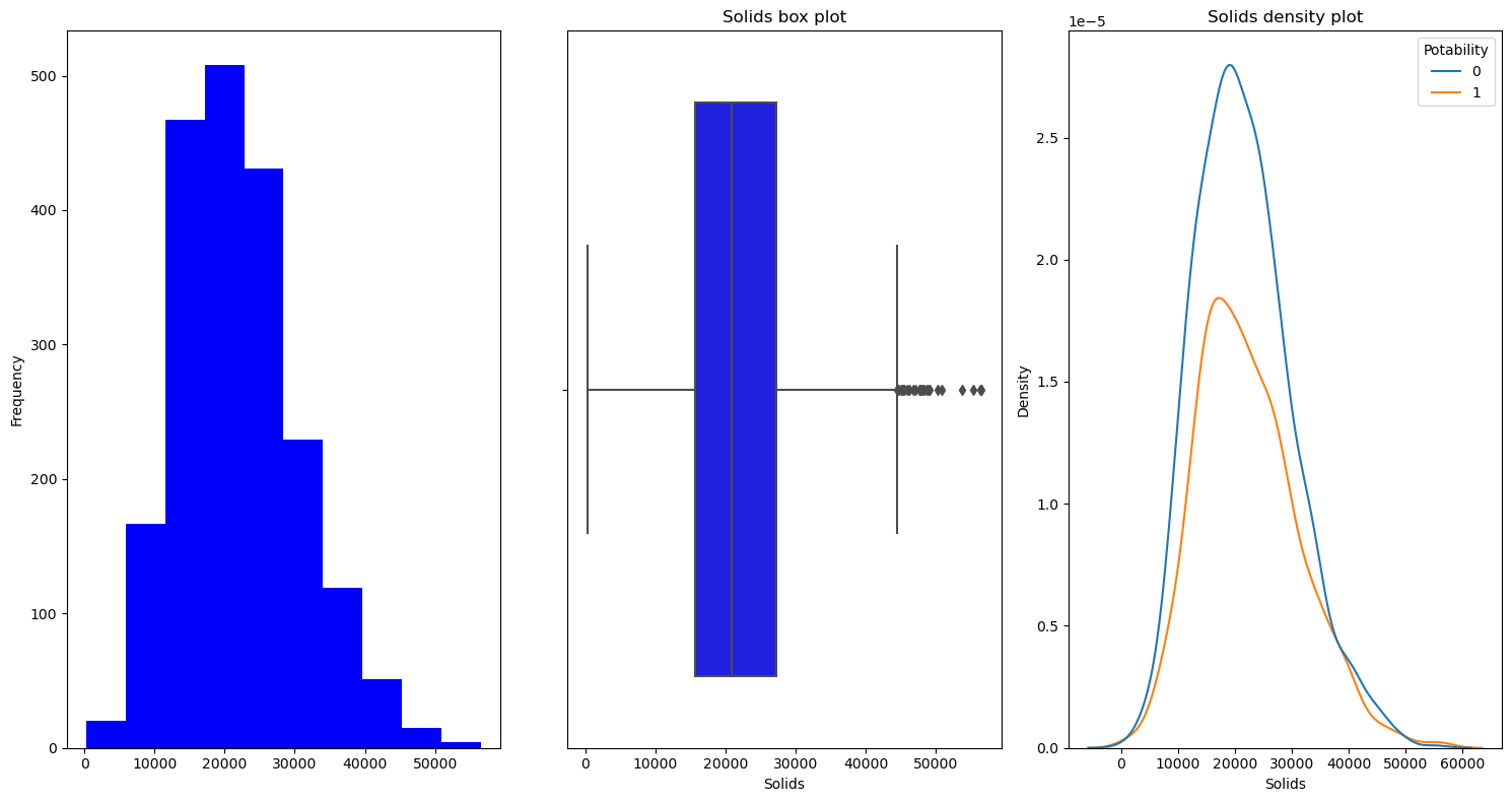
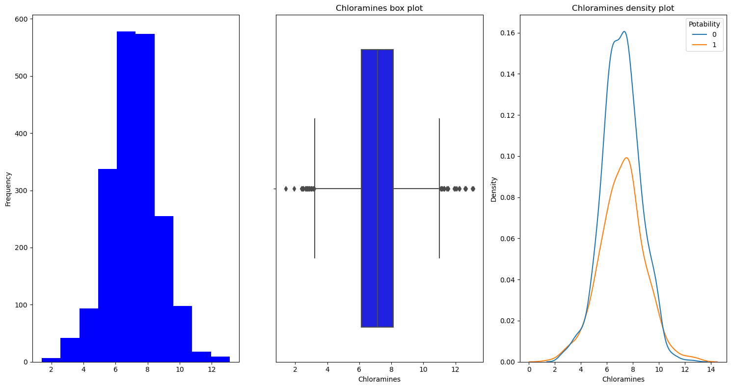
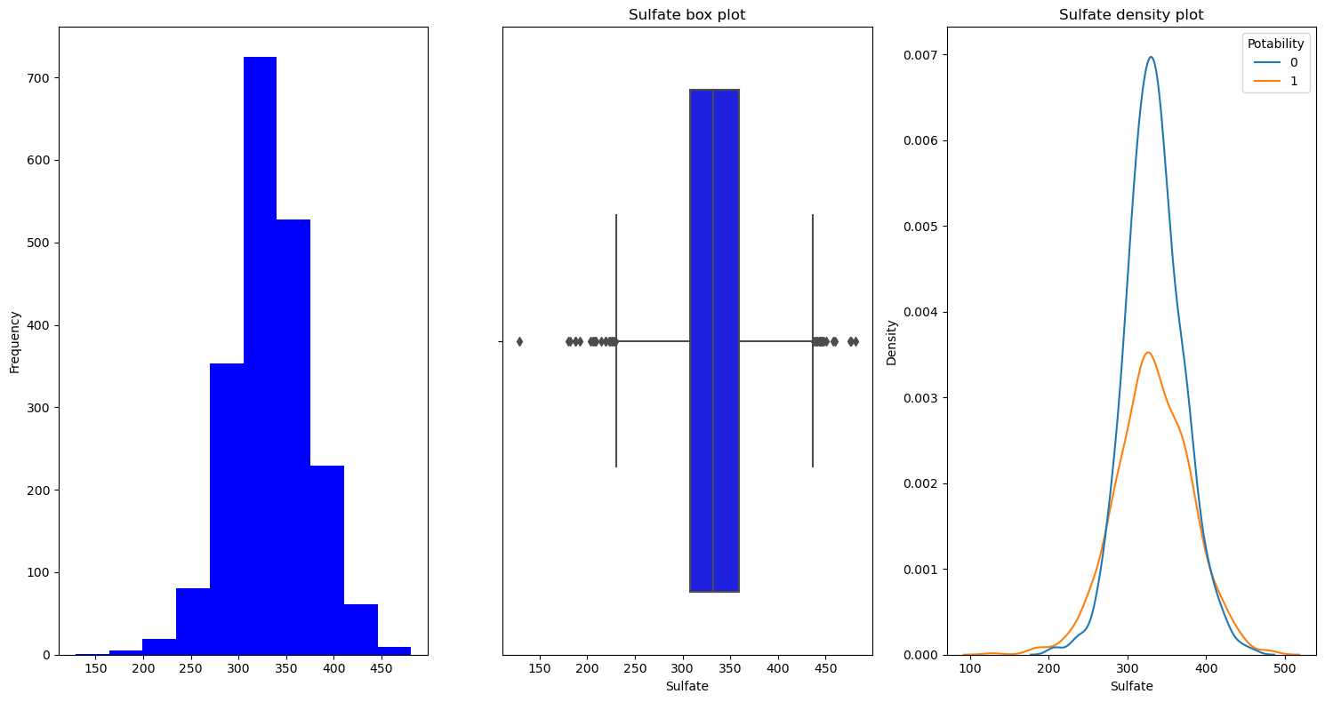
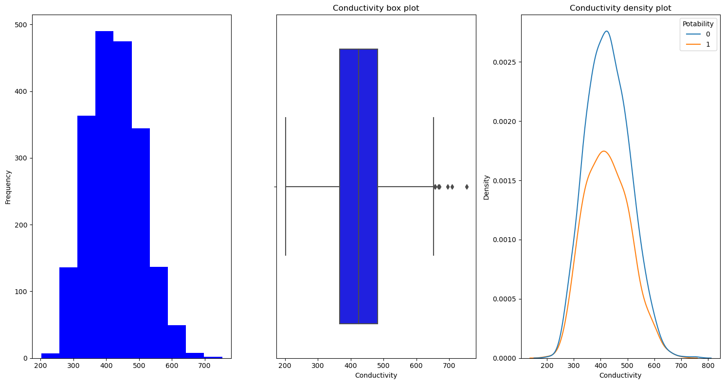
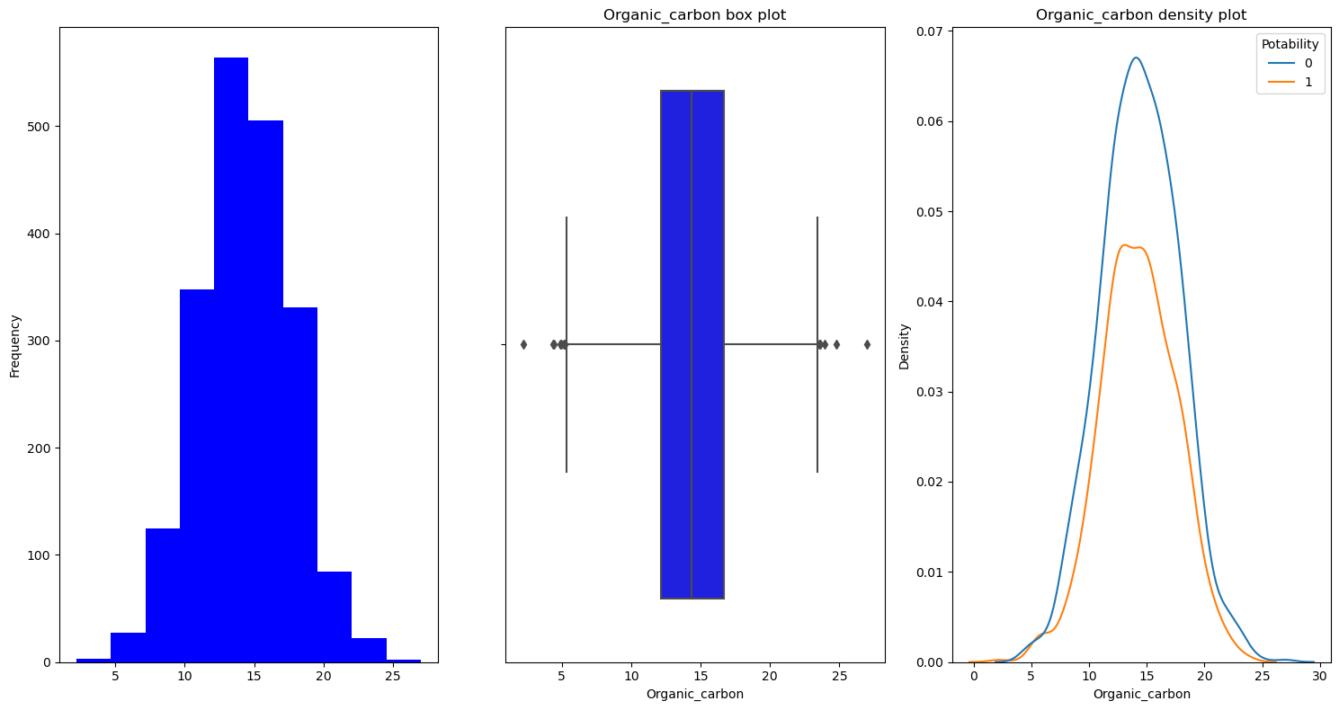
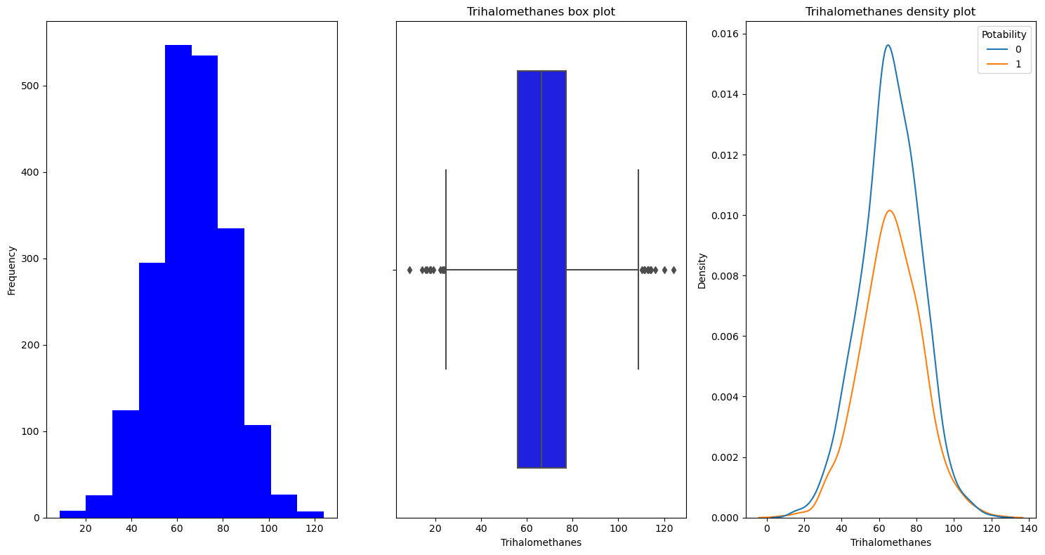
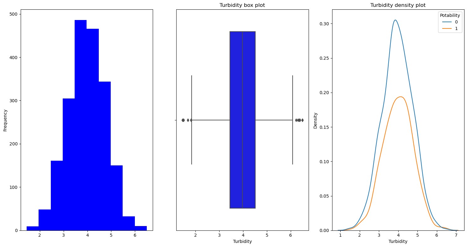
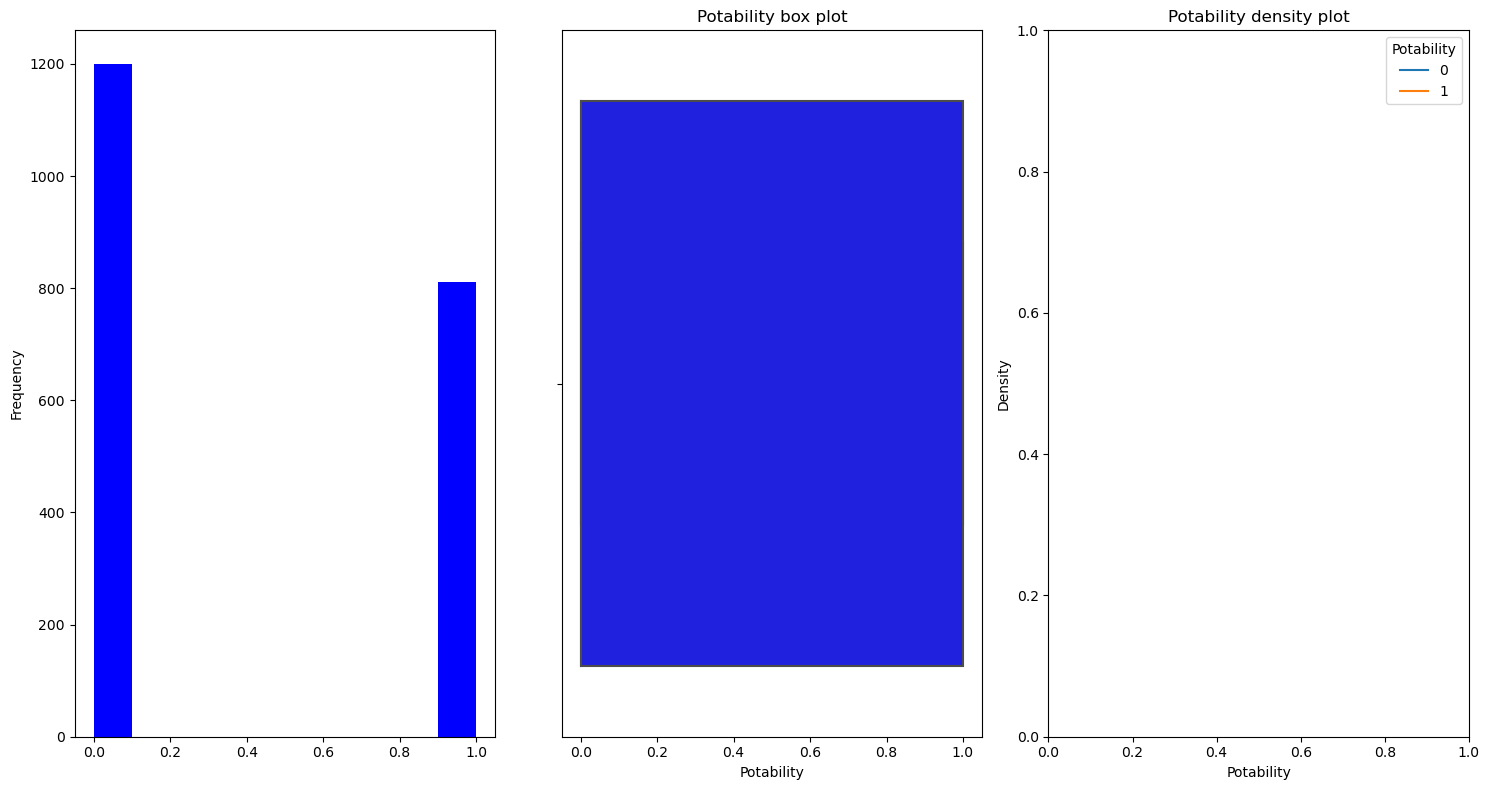
히스토그램과 박스차트, 그리고 밀도함수를 이용하여 데이터를 시각화해주는
feature_viz 함수를 생성했다.
히스토그램, 박스차트, 밀도함수
# 히스토그램, 박스 차트, 밀도 함수
plt.style.use('default')
def feature_viz(feature):
    plt.figure(figsize=(15,8))
    plt.title(f'{feature} hist plot')
    plt.subplot(1,3,1)
    df[feature].plot(kind='hist', color='b')

    plt.subplot(1,3,2)
    plt.title(f'{feature} box plot')
    sns.boxplot(df[feature], hue=df['Potability'], color='blue')

    plt.subplot(1, 3, 3)
    plt.title(f'{feature} density plot')
    sns.kdeplot(df[feature], hue=df['Potability'])
    plt.tight_layout()
plt.style.use('default')
for i in df.columns:
feature_viz(i)Ph
Hardness

Solids
Chioramines
Sulfate
Conductivity
Organic_carbon
Trihalomethanes
Turbidity
Potability
독립변수 히스토그램
#독립변수 히스토그램
plt.style.use('default')
fig, ax =plt.subplots(9,1,figsize=(20,100))
x=0
for i in range(0, 9):
    sns.histplot(x=df.columns[x], data=df, hue='Potability', ax=ax[i]);
    ax[i].set_title(df.columns[x])
    fig.show()
    x+=1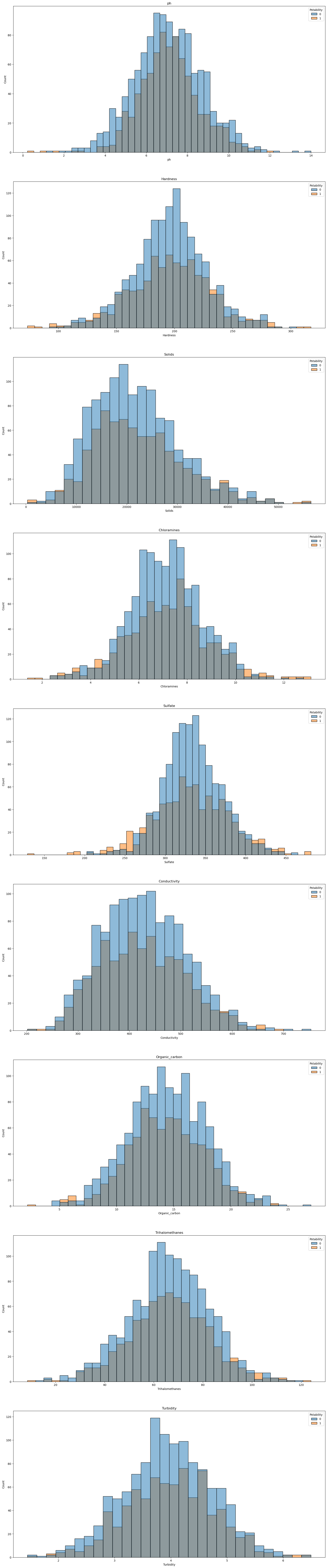
뭔가 양 사이드에서 식수가 많이 보이는 것 같다.
높던지 낮던지 해야하는 걸까..
계속 해보자.
산점도 행렬
# 산점도 행렬
sns.pairplot(df, hue="Potability", markers=["o", "s"])
plt.title("Water Quality Corrplot")
plt.show()
으으 눈아파
상관행렬
# 상관 행렬
plt.figure(figsize = (8,8))
sns.heatmap(df.corr(), cmap= 'Spectral', annot=True, square=True)
상관도가 다들 형편이 없다.
왜 그럴까 ..? ㅠ
상관계수가 낮아도 랜덤포레스트 등 머신러닝 모델들의 정확도는 높은 사례는 매우 빈번하다고 한다.
그냥 가보자.
이제 X,Y 로 각각 변수들을 분리시켜주자.
우리의 Target 은 Potability.
# 독립변수와 종속변수 X, y에 각각 분할
X = df.drop("Potability", axis = 1)
y = df['Potability']
# X에 따른 target의 분포 (strip)
plt.style.use('fivethirtyeight')
plt.figure(figsize = (20, 20))
for n, column in enumerate(X.columns):
plt.subplot(4, 3, n + 1)
sns.stripplot(x = y , y = X[column], size = 4)
X에 따른 target 의 분포를 알아보자.

진짜 다 똑같이 생긴 것 같다.
뭔가 얻은 게 없다.. 내 눈에는.
Boxen 을 이용해서 확인해보자.
# X에 따른 target의 분포 (Boxen)
plt.figure(figsize = (20, 20))
for n, column in enumerate(X.columns):
    plt.subplot(4, 3, n + 1)
    sns.boxenplot(x = y , y = X[column])
다를 바가 없는 것 같다.
0과 1사이의 차이도 크게 없는 것 같다.
그나마 조금 보이는 것은 Sulfate 에서 중앙값에 있는 데이터가 1이 좀 많다..? 는 것..?
plt.figure(figsize = (20, 20))
for n, column in enumerate(X.columns):
    plt.subplot(4, 3, n + 1)
    sns.distplot(X[column], color = 'r')
내 눈에는 크게 뭔가 보이지 않는다.
데이터 전처리 (Preprocessing)
표준화
표준화를 진행해줄 것이다.
머신러닝 모델들에는 데이터 표준화에 민감하게 학습되는 알고리즘들이 있다.
KNN, SVM, Logistic Regression(로지스틱 회귀) 등은 표준화에 민감하게 반응하기 때문에
예측 모델링을 하기 전에 데이터 표준화를 진행해주는 것이 성능이 좋다.
Target 데이터를 제외한 X 데이터들을 표준화시켜주자.

표준화 전 데이터
StandardSclaer 를 사용해서 표준화시켜주었다.
from sklearn.preprocessing import StandardScaler
st = StandardScaler()
col= X.columns
X[col] = st.fit_transform(X[col])
X[col]
표준화가 이루어졌다.
위의 탐색적 데이터분석에서 알아보았을 때,
Potability 데이터의 0과 1 . 데이터들의 수가 차이가 나는 것을 확인했었다.
불균형 데이터라는 것이다.
오버샘플링을 해주는 것이 필요할 것 같다.
근데,
만약 오버샘플링을 하지 않는다면 어떻게 될까?
궁금하니 직접 데이터를 학습시켜서 확인해보자.
오버샘플링 이전 학습
# 업샘플링없이 학습/검증 분할
X_train, X_test, y_train, y_test = train_test_split(X, y, test_size = 0.2, stratify=y)
X_train.shape, y_train.shape
((1608, 9), (1608,))8:2 로 Train, Test 데이터를 분류해주었다.
# 클래스 빈도
y_train.value_counts()
0 960
1 648
Name: Potability, dtype: int64# test data 클래스 빈도
y_test.value_counts()0 240
1 163
Name: Potability, dtype: int64데이터가 나뉜 것을 확인해주고,
학습시켜보자.
# 업샘플링 전 랜덤 포레스트
from sklearn.ensemble import RandomForestClassifier
import time
start = time.time()
rnd_clf = RandomForestClassifier()
rnd_clf.fit( X_train, y_train ) #학습
rnd_clf_pred = rnd_clf.predict(X_test) #X_test 예측
rnd_clf_acc = rnd_clf.score(X_test, y_test) # 정확도(Accuracy) 출력
print("랜덤포레스트 training accuracy  :", rnd_clf.score(X_train, y_train)*100, "%")
print("랜덤포레스트 test accuracy :", rnd_clf_acc * 100, "%")
end = time.time()
print('Execution time is:', end - start)
랜덤포레스트 training accuracy : 100.0 %
랜덤포레스트 test accuracy : 66.74937965260546 %
Execution time is: 0.38340306282043457
잉, 트레이닝 정확도가 100% 라면 학습이 엄청 잘 된 건데
Test 정확도는 67%밖에 나오지 않았다.
정확도가 높지 않은 모델이 만들어지는 것이다.
그렇다면, 오버샘플링을 한다면?
오버샘플링을 해주기 이전,
오버샘플링에 대한 설명은 여기를 참조하자.
https://wndofla123.tistory.com/31
Python으로 배우는 데이터 전처리 이해(II) - 불균형 데이터 처리(Imbalanced Data) - 오버 샘플링(Over Sam
Intro 이전 게시물 https://wndofla123.tistory.com/30 공공빅데이터 청년인턴/데이터Python으로 배우는 데이터 전처리 이해(II) - 불균형 데이터 처리(Imb Intro 데이터 전처리 과정에서 분석 변수 처리 과정에..
wndofla123.tistory.com
오버샘플링 - SMOTE
SMOTE 를 사용해서 학습시켜보자.
SMOTE 는 소수클래스에 속하는 데이터 주변에 원본 데이터와 동일하지는 않으면서
소수 클래스에 해당하는 가상의 데이터를 생성해서 데이터를 증식시킨다.
# SMOTE 오버샘플링
from imblearn.over_sampling import SMOTE
oversample = SMOTE()
X_up, y_up = oversample.fit_resample(X, y)
print(X_up.shape) # 입력데이터 행열 확인
print(y_up.value_counts()) # 출력데이터 클래스 빈도 확인
(2400, 9)
0 1200
1 1200
Name: Potability, dtype: int64개수가 잘 맞춰졌다.
# 오버샘플링 후 학습/검증 분할
X_train, X_test, y_train, y_test = train_test_split(X_up, y_up, test_size = 0.2, stratify=y_up)
print(X_train.shape) # 입력데이터 행열 확인
print(y_train.value_counts()) # 출력데이터 클래스 빈도 확인
# SMOTE 오버샘플링 후 split - modeling
rnd_clf = RandomForestClassifier()
rnd_clf.fit( X_train, y_train ) #학습
rnd_clf_pred = rnd_clf.predict(X_test) #X_test 예측
rnd_clf_acc = rnd_clf.score(X_test, y_test) # 정확도(Accuracy) 출력
print("랜덤포레스트 training accuracy :", rnd_clf.score(X_train, y_train)*100, "%")
print("랜덤포레스트 test accuracy :", rnd_clf_acc * 100, "%")랜덤포레스트 training accuracy : 100.0 % 랜덤포레스트 test accuracy : 70.83333333333334 %70.83
3퍼정도 올랐다.
하찮다.
다른 오버샘플링도 진행해보자.
오버샘플링 - ADASYN
보더라인 스모트와 비슷한 형식이지만, 샘플링 개수를 데이터 위치에 따라 다르게 설정하는 방법이다.
밀도를 기반으로 한다.
# ADASYN 오버 샘플링
from imblearn.over_sampling import ADASYN
oversample = ADASYN()
X_up_ada, y_up_ada = oversample.fit_resample(X, y)
print(X_up_ada.shape)
print(y_up_ada.value_counts())
(2487, 9)
1 1287
0 1200
Name: Potability, dtype: int64완전히 똑같이 하지는 않나보다.
# ADASYN 오버샘플링 후 split - modeling
X_train_ada, X_test_ada, y_train_ada, y_test_ada = train_test_split(X_up_ada, y_up_ada,
                                                    test_size = 0.2, stratify=y_up_ada)

rnd_clf = RandomForestClassifier()
rnd_clf.fit( X_train_ada, y_train_ada ) #학습
rnd_clf_pred = rnd_clf.predict(X_test_ada) #X_test 예측
rnd_clf_acc = rnd_clf.score(X_test_ada, y_test_ada) # 정확도(Accuracy) 출력
print("랜덤포레스트 training accuracy  :", rnd_clf.score(X_train_ada, y_train_ada)*100, "%")
print("랜덤포레스트 test accuracy :", rnd_clf_acc * 100, "%")
랜덤포레스트 training accuracy : 100.0 %
랜덤포레스트 test accuracy : 76.30522088353415 %76% 로 뛰었다 !
상당히 정확도가 나쁘지 않다.
오버샘플링 - RandomOverSampler
그렇다면 RandomOverSampler 는 ?
# RandomOverSampling
from imblearn.over_sampling import RandomOverSampler
oversample = RandomOverSampler()
X_up_ROS, y_up_ROS = oversample.fit_resample(X, y)
print(X_up_ROS.shape)
print(y_up_ROS.value_counts())
(2400, 9)
0 1200
1 1200
Name: Potability, dtype: int64# RandomOverSampler 오버샘플링 후 split - modeling
X_train_ROS, X_test_ROS, y_train_ROS, y_test_ROS = train_test_split(X_up_ROS, y_up_ROS,
test_size = 0.2, stratify=y_up_ROS)
from sklearn.ensemble import RandomForestClassifier
rnd_clf = RandomForestClassifier()
rnd_clf.fit( X_train_ROS, y_train_ROS ) #학습
rnd_clf_pred = rnd_clf.predict(X_test_ROS) #X_test 예측
rnd_clf_acc = rnd_clf.score(X_test_ROS, y_test_ROS) # 정확도(Accuracy) 출력
print("랜덤포레스트 training accuracy :", rnd_clf.score(X_train_ROS, y_train_ROS)*100, "%")
print("랜덤포레스트 test accuracy :", rnd_clf_acc * 100, "%")랜덤포레스트 training accuracy : 100.0 %
랜덤포레스트 test accuracy : 75.20833333333333 %오..
ADASYN 이 제일 높은 정확도를 보여주었다.
얘로 가보자고.
학습/검증 데이터는 ada 데이터로 해줘야 하지만....
코치님은 RandomOverSampler 로 해주었으므로
나도 RandomOversampler 데이터로 해줘야지.
코치님 결과와 다르다. 무섭다
분류모델링
랜덤포레스트는 이미 튜닝 없이 76.3% 의 정확도를 보여주었기 때문에,
오차행렬은 따로 확인하지 않고 파라미터를 튜닝해주기 위해 GridSearchCV 로 넘어갔다.
GridSearchCV 는 하이퍼 파라미터 설정에 도움을 주어, 효과적으로 모델의 성능을 높이는 데
도움을 준다.
랜덤 포레스트
from sklearn.model_selection import GridSearchCV
start = time.time()
rnd_clf = RandomForestClassifier()
param_grid = { 'n_estimators':[100,200, 350, 500],
               'min_samples_leaf':[2, 10, 30]}

gscv_rnd = GridSearchCV(rnd_clf, param_grid,cv=5)
gscv_rnd.fit(X_train_ROS, y_train_ROS)
print("랜덤포레스트 최적 점수 : {}".format(gscv_rnd.best_score_))
print("랜덤포레스트 최적 파라미터 : {}".format(gscv_rnd.best_params_))

print(gscv_rnd.best_estimator_)
end = time.time()
print('Execution time is:')
print(end - start)
랜덤포레스트 최적 점수 : 0.7369791666666667
랜덤포레스트 최적 파라미터 : {'min_samples_leaf': 2, 'n_estimators': 200}
RandomForestClassifier(min_samples_leaf=2, n_estimators=200)
Execution time is:
45.73830842971802위에서 나온 파라미터대로 하이퍼 파라미터를 설정해서
모델 안에 넣어주었다.
plt.style.use('default')
start = time.time()
rnd_clf = RandomForestClassifier(min_samples_leaf=2, n_estimators=350, random_state=42)
rnd_clf.fit( X_train_ROS, y_train_ROS ) #학습
rnd_clf_pred = rnd_clf.predict(X_test_ROS) #X_test 예측
rnd_clf_acc = rnd_clf.score(X_test_ROS, y_test_ROS) # 정확도(Accuracy) 출력
print("랜덤포레스트 training accuracy  :", rnd_clf.score(X_train_ROS, y_train_ROS)*100, "%")
print("랜덤포레스트 test accuracy :", rnd_clf_acc * 100, "%")
print("--------------------------------------------------------------------------")
print(classification_report(y_test_ROS, rnd_clf_pred))
print("--------------------------------------------------------------------------")
print(confusion_matrix(y_test_ROS, rnd_clf_pred))
print("--------------------------------------------------------------------------")
end = time.time()
print('Execution time is:')
print(end - start)
plot_confusion_matrix(rnd_clf, X_test_ROS, y_test_ROS, cmap='YlGn')
plt.title("<< Random Forest >>")
랜덤포레스트 training accuracy : 99.84375 %
랜덤포레스트 test accuracy : 77.29166666666667 %
--------------------------------------------------------------------------
precision recall f1-score support
0 0.77 0.78 0.78 240
1 0.78 0.76 0.77 240
accuracy 0.77 480
macro avg 0.77 0.77 0.77 480
weighted avg 0.77 0.77 0.77 480
--------------------------------------------------------------------------
[[188 52]
[ 57 183]]
--------------------------------------------------------------------------
Execution time is:
1.507847547531128
77.3 퍼센트 정도의 정확도를 보인다.
(혹시나 해서 ada 데이터를 넣었을 때는 파라미터는 똑같이 나왔는데,
파라미터를 넣으니 정확도가 75.1%가 나왔다. 그냥 코치님 하신 대로 ROS데이터를 사용하자)
변수중요도를 보자.
# 변수 중요도 Series 생성 후 sorting
forest_importances = pd.Series(rnd_clf.feature_importances_)
feature_scores = pd.Series(rnd_clf.feature_importances_, index=X_train.columns).sort_values(ascending=False)
feature_scores
# 변수 중요도 seaborn bar plot
f, ax = plt.subplots(figsize=(15, 10))
ax = sns.barplot(x=feature_scores, y=feature_scores.index)
ax.set_title("Visualize feature scores of the features")
ax.set_xlabel("Feature importance score")
ax.set_ylabel("Features")
plt.show()
Sulfate와 Ph 가 꽤나 중요한 변수이다.
로지스틱 회귀
from sklearn.model_selection import GridSearchCV
from sklearn.linear_model import LogisticRegression
import numpy as np

lr = LogisticRegression( random_state = 0 )

params = {'C' : [0.1, 1, 3, 5, 10],
          'max_iter' : [10, 100, 1000],
          "penalty":["l1","l2"]
          }
lr_grid_cv = GridSearchCV(lr, param_grid=params, cv=3, scoring='accuracy', verbose=1)
import time
start = time.time()
#----------------------------------------------
lr_grid_cv.fit( X_test_ROS , y_test_ROS)
print("로지스틱 최적 점수 : {}".format(lr_grid_cv.best_score_))
print("로지스틱 최적 파라미터 : {}".format(lr_grid_cv.best_params_))
print(lr_grid_cv.best_estimator_)
#----------------------------------------------
end = time.time()
print("--------------------------------------------------------------------------")
print('Execution time is:')
print(end - start)Fitting 3 folds for each of 30 candidates, totalling 90 fits
로지스틱 최적 점수 : 0.4916666666666667
로지스틱 최적 파라미터 : {'C': 0.1, 'max_iter': 10, 'penalty': 'l2'}
LogisticRegression(C=0.1, max_iter=10, random_state=0)
--------------------------------------------------------------------------
Execution time is:
0.21210980415344238위에서 나온 파라미터를 기준으로 하이퍼파라미터를 설정해서 로지스틱 회귀를 진행해주자.
from sklearn.linear_model import LogisticRegression
### 로지스틱 회귀 ###
start = time.time()
#----------------------------------------------
lr = LogisticRegression(C=3, max_iter=1000, random_state=0)
lr.fit( X_train_ROS, y_train_ROS )
lr_pred = lr.predict( X_test_ROS )
lr_acc = lr.score( X_test_ROS, y_test_ROS )
#----------------------------------------------
print("로지스틱 회귀 training accuracy :", lr.score( X_train_ROS, y_train_ROS )*100, "%")
print("로지스틱 회귀 testing accuracy :", lr_acc * 100, "%")
print("--------------------------------------------------------------------------")
print(classification_report( y_test_ROS, lr_pred ))
print("--------------------------------------------------------------------------")
print(confusion_matrix( y_test_ROS, lr_pred ))
print("--------------------------------------------------------------------------")
#----------------------------------------------
end = time.time()
print('로지스틱 회귀 수행시간 :')
print(end - start)
plt.figure(figsize=(20, 20))
plot_confusion_matrix(lr , X_test_ROS , y_test_ROS , cmap='Blues')
LGBM
from lightgbm import LGBMClassifier

lgbm = LGBMClassifier(n_estimators=1000)

# 조기 중단 기능에 필요한 파라미터 정의
evals = [(X_test_ROS, y_test_ROS)]
lgbm.fit(X_train_ROS, y_train_ROS, eval_metric='logloss', eval_set=evals, verbose=True)
lgbm_pred = lgbm.predict(X_test_ROS)
pred_proba = lgbm.predict_proba(X_test_ROS)[:,1]
lgbm_acc = lgbm.score(X_test_ROS, y_test_ROS)
print("Light GBM training accuracy :", lgbm.score(X_train_ROS, y_train_ROS)*100, "%")
print("Light GBM testing accuracy :", lgbm_acc * 100, "%")
print("--------------------------------------------------------------------------")
print(classification_report(y_test_ROS, lgbm_pred))
print("--------------------------------------------------------------------------")
print(confusion_matrix(y_test_ROS, lgbm_pred))
print("--------------------------------------------------------------------------")
plot_confusion_matrix(lgbm, X_test_ROS, y_test_ROS, cmap='Purples')
end = time.time()
print("--------------------------------------------------------------------------")
print('Execution time is:')
print(end - start)
plt.title("<< Light GBM >>")
Light GBM training accuracy : 100.0 %
Light GBM testing accuracy : 73.54166666666667 %
--------------------------------------------------------------------------
precision recall f1-score support
0 0.74 0.72 0.73 240
1 0.73 0.75 0.74 240
accuracy 0.74 480
macro avg 0.74 0.74 0.74 480
weighted avg 0.74 0.74 0.74 480
--------------------------------------------------------------------------
[[172 68]
[ 59 181]]
--------------------------------------------------------------------------
--------------------------------------------------------------------------
Execution time is:
0.9527244567871094
lgbm.feature_importances_
lgbm_feature_scores = pd.Series(lgbm.feature_importances_, index=X_train.columns).sort_values(ascending=False)
# Creating a seaborn bar plot

f, ax = plt.subplots(figsize=(15, 10))
ax = sns.barplot(x=lgbm_feature_scores, y=lgbm_feature_scores.index)
ax.set_title("LightGBM feature scores of the features")
ax.set_xlabel("Feature importance score")
ax.set_ylabel("Features")
plt.show()
SV 서포트 벡터 머신
from sklearn.model_selection import GridSearchCV
from sklearn.svm import SVC
start = time.time()
# defining parameter range
param_grid = {'C': [0.1, 1, 10, 100, 1000],
              'gamma': [1, 10, 30, 50, 70],
              'kernel': ['rbf']}

grid = GridSearchCV(SVC(), param_grid, refit = True, verbose = 3)

# fitting the model for grid search
grid.fit(X_train_ROS, y_train_ROS)
end = time.time()
print('Execution time is:', end - start)

print("SVM 최적 점수 : {}".format(grid.best_score_))
print("SVM 최적 파라미터 : {}".format(grid.best_params_))
print(grid.best_estimator_)
SVM 최적 점수 : 0.7083333333333333
SVM 최적 파라미터 : {'C': 1, 'gamma': 10, 'kernel': 'rbf'}
SVC(C=1, gamma=10)
### 서포트 벡터 머신 ###
from sklearn.svm import SVC
import time
start = time.time()
#----------------------------------------------
svm_clf = SVC( C=1, gamma=10, random_state=0 )
svm_clf.fit( X_train_ROS, y_train_ROS )
svm_pred = svm_clf.predict( X_test_ROS )
svm_acc = svm_clf.score( X_test_ROS ,  y_test_ROS )
#----------------------------------------------
print("SVM training accuracy :", svm_clf.score( X_train_ROS , y_train_ROS )*100, "%")
print("SVM testing accuracy :", svm_acc * 100, "%")
#----------------------------------------------
print("--------------------------------------------------------------------------")
print(classification_report(y_test_ROS , svm_pred))
print("--------------------------------------------------------------------------")
print(confusion_matrix(y_test_ROS , svm_pred))
print("--------------------------------------------------------------------------")
#----------------------------------------------
plot_confusion_matrix(svm_clf, X_test_ROS,  y_test_ROS, cmap='Oranges')
plt.title("<< Support Vector Machine >>")

end = time.time()
print('Execution time is:')
print(end - start)
SVM training accuracy : 100.0 %
SVM testing accuracy : 76.875 %
--------------------------------------------------------------------------
precision recall f1-score support
0 0.68 1.00 0.81 240
1 1.00 0.54 0.70 240
accuracy 0.77 480
macro avg 0.84 0.77 0.76 480
weighted avg 0.84 0.77 0.76 480
--------------------------------------------------------------------------
[[240 0]
[111 129]]
--------------------------------------------------------------------------
Execution time is:
0.7000243663787842
지금까지 학습시켰던 4개 모델의 정확도를 데이터프레임으로 그려서 확인해보고,
시각화해서 확인해보자.
# Accuracy 데이터 프레임 생성
models_acc = {'Logistic Regression': lr_acc*100,
              'SVM': svm_acc*100,
              'LighGBM':lgbm_acc*100 ,
              'Random Forest': rnd_clf_acc*100
              }

models_acc_df = pd.DataFrame(pd.Series(models_acc))
models_acc_df.columns = ['정확도']
models_acc_df['모델'] = ['Logistic Regression', 'SVM',
                          'LighGBM', 'Random Forest']
models_acc_df.set_index(pd.Index([1, 2 , 3 , 4 ]))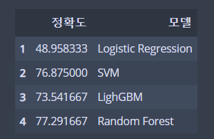
plt.figure(figsize=[14, 8])
axis = sns.barplot(x = '모델', y = '정확도', data = models_acc_df, palette="flare")
axis.set(xlabel='< Classifiers >', ylabel='< Accuracy >', ylim=(50, 90),)

for p in axis.patches:
    height = p.get_height()
    axis.text(p.get_x() + p.get_width()/2, height + 0.005, '{:1.2f}%'.format(height), ha="center" ,fontsize = 20)

plt.title("<< Classifier Accuracy Comparison >>", fontsize = 20)
랜포가 해냈다.
이제 이 랜덤포레스트 모델을 사용해서
Raw 데이터에 대입해보자.
모델 대입 - Raw Data 예측
우리가 지금까지 오버샘플링한 데이터로 모델에 학습 / 검증을 수행했고,
정확도를 위해 모델에 GridSearchCV를 적용하여 파라미터도 튜닝해주었다.
결과적으로 랜덤 포레스트 모델이 가장 성능이 좋은 것을 확인했다.
이제는 이 모델을 Raw Data 에 넣어 이 모델이 데이터를 잘 분류해주는 지를 확인해보자.


rnd_clf_pred = rnd_clf.predict( X ) #X_test 예측
rnd_clf_acc = rnd_clf.score( X , y ) # 정확도(Accuracy) 출력
print("랜덤포레스트 Raw data Prdict accuracy :", rnd_clf_acc * 100, "%")
print("--------------------------------------------------------------------------")
print(classification_report(y, rnd_clf_pred))
print("--------------------------------------------------------------------------")
print(confusion_matrix(y, rnd_clf_pred))
print("--------------------------------------------------------------------------")
end = time.time()
print('Execution time is:')
print(end - start)
plot_confusion_matrix(rnd_clf, X, y, cmap='magma' )
plt.title("<< Predict Raw data (Random Forest) >>")
랜덤포레스트 Raw data Prdict accuracy : 94.6295375435107 %
--------------------------------------------------------------------------
precision recall f1-score support
0 0.95 0.96 0.96 1200
1 0.93 0.93 0.93 811
accuracy 0.95 2011
macro avg 0.94 0.94 0.94 2011
weighted avg 0.95 0.95 0.95 2011
--------------------------------------------------------------------------
[[1147 53]
[ 55 756]]
--------------------------------------------------------------------------
Execution time is:
1.2193751335144043우왕 94% 의 높은 예측 정확도를 보였다 !

Review
왜인지 코치님이 하신 것보다 더 높은 (근데 진짜 왜지?) 성능의 모델을 얻었다.
근데 중간에 왜 ADASYN 의 성능이 더 높게 나왔는데 모델 돌리니 RandomOverSampling 해준 데이터보다
성능이 안 좋게 나왔는 지 이유를 모르겠다.
프로젝트 때 제대로 EDA 를 못 한 것 같아서 아쉬움이 남았다....
이거 먼저 해보고 프로젝트 들어갈걸.
그리고 나도 프로젝트때 똑같이 RandomForest 모델을 사용해서 변수 중요도를
뽑아냈었는데 , 그 때 아다리가 잘 맞아서 하이퍼 파라미터를 잘 조절해서 정확도가 0.91이 나왔었다.
GridSearchCV 를 알게 되었으니, 다음부터는 모델의 하이퍼 파라미터를 적용시켜서
모델 성능을 개선시킬 때 이 파라미터 조정 라이브러리를 알았으니 이거 써야지.
머신러닝 공부를 더 해야겠다.
미니 프로젝트 꿀잼

공빅 원주 기술코치 박성호님의 멋진 미니프로젝트 글을 참조했습니다 !
덕분에 공부 엄청 많이 되는 중 ㅠ
원주 기코님 최고
'Data Science > Machine Learning' 카테고리의 다른 글
| [Python/MachineLearning] 앙상블 알고리즘 (Ensemble Algorithms) : 보팅 (Votting) (2) | 2022.08.22 |
|---|---|
| [Python/MachineLearning] 앙상블 알고리즘 (Ensemble Algorithms) : 배깅 (Bagging) (2) | 2022.08.21 |
| [Python/MachineLearning] Boston Housing Price Data 를 이용한 Decision Tree 실습 (2) | 2022.08.15 |
| [Python/MachineLearning] Decision Tree(의사결정나무) (2) | 2022.08.15 |
| [Python/ML] K-NN (K-Nearest Neigthbor , K-최근접이웃) (1) | 2022.08.06 |


