
| 일 | 월 | 화 | 수 | 목 | 금 | 토 |
|---|---|---|---|---|---|---|
| 1 | 2 | 3 | 4 | |||
| 5 | 6 | 7 | 8 | 9 | 10 | 11 |
| 12 | 13 | 14 | 15 | 16 | 17 | 18 |
| 19 | 20 | 21 | 22 | 23 | 24 | 25 |
| 26 | 27 | 28 | 29 | 30 |
- NLP
- 오버샘플링
- datascience
- 2023공빅데
- 공빅
- 분석변수처리
- 데이터전처리
- 데이터분석
- 클러스터링
- data
- textmining
- machinelearning
- ADSP
- 공공빅데이터청년인재양성
- decisiontree
- Kaggle
- Keras
- 공빅데
- 빅데이터
- 2023공공빅데이터청년인재양성
- ADsP3과목
- DL
- 2023공공빅데이터청년인재양성후기
- DeepLearning
- SQL
- 텍스트마이닝
- 공공빅데이터청년인턴
- ML
- k-means
- 머신러닝
- Today
- Total
愛林
[Python/DL] 분류 알고리즘 (Classification Algorithm) : 인공신경망 (ANN : Article Neural Network) - (2) 본문
[Python/DL] 분류 알고리즘 (Classification Algorithm) : 인공신경망 (ANN : Article Neural Network) - (2)
愛林 2022. 12. 9. 09:39https://wndofla123.tistory.com/84
[Python/ML] 분류 알고리즘 (Classification Algorithm) : 인공신경망 (ANN : Article Neural Network)
2022.12.07 + 교육 내용 추가 인공신경망 (Article Neural Network : ANN) 인공신경망이란, 인간 뇌를 기반으로 한 추론 모델이다. 뉴런을 기본적인 정보처리 단위로 하여 만든 시스템이다. 인간의 뇌는 100억
wndofla123.tistory.com
(이전글)
인공신경망 (ANN) 실습

Tensorflow 를 사용하여 인공신경망을 만드는 실습을 진행해보자.
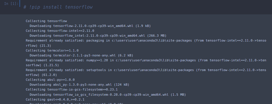
나는 Tensorflow 를 한 번도 사용해본 적이 없어서 !pip install Tensorflow 로 설치부터 해주었다.
sklearn 에서 제공해주는 dataset인 iris 데이터를 사용했다.
먼저 필요한 library 들을 import 해주었다.
import numpy as np
import pandas as pd
import matplotlib.pyplot as plt
import seaborn as sns
from sklearn.datasets import load_iris
from sklearn.model_selection import train_test_split
import tensorflow as tf
from tensorflow.keras.models import Sequential
from tensorflow.keras.layers import Dense
iris 데이터셋을 불러와주고, train_test_split 을 이용하여 train과 test셋을 분리해주었다.
# 데이터 불러오기
iris = load_iris()
df = pd.DataFrame(data = iris.data, columns = iris.feature_names)
df['label'] = iris.target

# 데이터 분할
y = df['label']
X = df.drop(['label'], axis= 1)

X_train, X_test, y_train, y_test = train_test_split(X, y, random_state = 42,
                                                   stratify = y)
                                             # stratify로 target 의 class를 유지한채로 분리
확인해주었다.
이제 ANN모델을 만들어볼 차례 ..
# model 설정
model = Sequential() # 모델을 직렬로 잇는다.
model.add(Dense(8, input_dim = 4, activation = 'relu')) # 레이어 객체를 인자로 넘겨 모델에 더한다.
# 8개의 노드, dim = 4가지 속성
model.add(Dense(3, activation = 'softmax')) # 분류이므로 softmax, 3개 노드
Sequential 을 통해서 모델을 이어준다.
Layer는 Dense 레이어를 사용했다. Target 변수를 제외하고 총 변수는 4개이므로 input_dim(dimension) 은 4.
활성화함수로는 ReLu 함수를 사용했다.
여기서 Dense 레이어란, 각 뉴런이 이전 계층의 모든 뉴런으로부터 입력을 받게 되는 것이다.
완전연결레이어 (Fully Connected Layer) Input과 Output을 모두 연결시켜준다.
추출된 정보들을 하나의 Layer로 모으고 이를 원하는 차원으로 축소시켜 표현하기 위한 레이어이다.
레이어를 구성하는 노드의 수인 unit은 8개,
다음 레이어는 3개를 사용했다. 이렇게 2개로 모델을 만들어주었다.
마지막 레이어는 분류문제이므로 활성화함수를 Softmax함수를 사용했다.
# 모델 컴파일
model.compile(loss = 'sparse_categorical_crossentropy',
             optimizer = 'adam',
             metrics = ['accuracy'])
모델을 컴파일해주었다.
손실함수는 sparse_categorical_crossentropy , 옵티마이저는 adam을 사용했다.
# 모델 실행
model.fit(X_train, y_train, epochs = 50, batch_size = 4)
모델을 피팅해주고 실행시켰다.
에폭이 50, 배치사이즈는 4. 학습횟수를 4개씩 50번 학습시킨다.

열심히 하는중
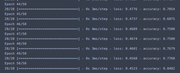
정확도가 점점 높아지는 것이 보이고 있다.
85%정도밖에 안 나ㅇ오넹

모델평가와 summary 까지 진행해주었다.
강의자료에선 되게 정확도가 높았던 것 같은데
내껀 별로 정확도가 높지 않다...
인공신경망의 성능을 개선시켜보자.
은닉층과 노드 수를 증사시킬수록 정확도는 높아지게 된다.
그렇지만 너무 정확도가 높을 시 과적합(Overfitting) 문제가 생길수 있으므로,
우리는 일반화가 잘 된 모델을 만드는 것이 중요하다.
◇ 일반화(Generalization) 모델을 만드는 방법
- 학습 데이터를 충분하게 늘린다.
-> 일반적으로 이미지 데이터를 분류할 때 사용한다. - 과적합이 발생하기 이전에 학습을 종료한다.
-> RandomForest 방법의 조기종료가 생각나는 방법.
적당히 학습시키고 만다. - 모델의 복잡도를 낮춘다.
-> L1, L2, Dropout 을 사용한다.
손실함수에 패털티를 주어 일부러 오차를 생성하거나,
학습 중 랜덤하게 노드를 꺼뜨린다.(Dropout)
과적합을 해결하기 위해서는 큰 가중치에 대해 큰 패널티를 부여해서 과적합을 예방하고,
데이터 값의 범위를 변환시켜 학습 결과가 특정 데이터 분포에 과적합될 가능성을 낮춘다.
정규화 방법으로는 Standardization, MinMax 정규화 등이 있다.
인공신경망에서만 사용되는 방법으로 Batch Normalization 이 있는데, 한 번에 입력으로 들어오는 배치 단위로
데이터 분포의 평균이 0, 분산이 1이 되도록 정규화하는 방법이다.
이 경우,
정규화된 데이터를 스케일 및 시프트하여 다음 레이어에 일정한 범위의 값들만 전달시킨다.
은닉층 단위마다 배치 정규화를 넣어주면 학습 전체 과정이 안정화되는 효과를 가져온다.
skelarn에서 제공해주는 load_boston 데이터셋을 이용하여 실습해보자.
from sklearn.datasets import load_boston

# 데이터 불러오기
boston = load_boston()
boston_df = pd.DataFrame(data = boston.data, columns = boston.feature_names)
boston_df['PRICE'] = boston.target
boston_df.head()
# 데이터 분할
y = boston_df['PRICE']
X = boston_df.drop(['PRICE'], axis = 1)

X_train, X_test, y_train, y_test = train_test_split(X,y, random_state = 42)

# 모델의 설정
model = Sequential()
model.add(Dense(16, input_dim = 13, activation = 'relu'))
model.add(Dense(1, activation ='relu'))
데이터를 분할해주고 모델을 만들어주었다.
활성화함수는 둘 다 relu함수를 사용했다. 분류가 아니고 예측이니까 .
# 모델 컴파일
model.compile(loss = 'mean_squared_error',
              optimizer = 'adam',
              metrics = ['mse'])

model.summary()
Model: "sequential_1"
_________________________________________________________________
Layer (type) Output Shape Param #
=================================================================
dense (Dense) (None, 16) 224
dense_1 (Dense) (None, 1) 17
=================================================================
Total params: 241
Trainable params: 241
Non-trainable params: 0
_________________________________________________________________모델을 컴파일 해보았다.
summary 로 모델을 살펴볼 수도 있다.
MSE 를 사용하고, 옵티마이저는 adam을 사용하여 컴파일 해주었다.
입력이 13개이고 출력이 17이면 221 아닌가요 왜 224 ? 17.몇몇이 224인데 아무튼 계산이 이상..
# 모델 실행
model.fit(X_train, y_train, epochs = 50, batch_size = 10)
모델을 실행해주었다.

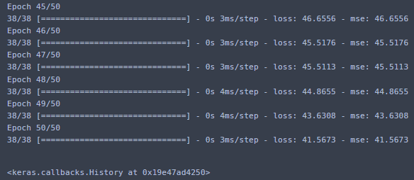
mse 가 갈수록 줄어드는 것을 확인할 수있다.
y_pred = model.predict(X_test)
y_pred[0]
array([28.251339], dtype=float32)0번째의예측값을 확인했을 때 28.25이다.

실제값은 24로 차이가 좀 있는 편.
plot 을 그려서 확인해보자.
history= model.fit(X_train, y_train, epochs = 500, verbose = 0, validation_split = 0.2)plot을 그리는 함수를 만들어주었다.
def plot_loss(history):
    plt.plot(history.history['loss'], label = 'loss')
    plt.plot(history.history['val_loss'], label = 'val_loss')
    plt.ylim([0,40])
    plt.xlabel("Epoch")
    plt.ylabel('Error')
    plt.legend()
    plt.grid(True)
plot_loss(history)
정규화를 시켜주지 않았더니 삐죽삐죽한 것을 확인할 수 있다.
이제 정규화를 진행해보자.
from tensorflow.keras.layers.experimental import preprocessing

normalizer = preprocessing.Normalization(axis = -1)
normalizer.adapt(np.array(X_train))

normalized_model = Sequential()
normalized_model.add(normalizer)
normalized_model.add(Dense(16,activation = 'relu'))
normalized_model.add(Dense(1, activation = 'relu'))

normalized_model.summary()
tensorflow 에서 제공해주는 preprocessing 을 사용하여 정규화시켜주었다.
Normalizer 를 만들어준 뒤, 이를 X_train에 적용시켜준다.
dataframe 상태로는 적용이 안 되니까 array로 바꾸어서 adapt 시켜주었다.
다음 이 Normalizer을 사용할 정규화모델을 만들어주었다.
모델에 Normalizer 를 낑꿔넣어준다.
나머지는
위에서 했던 방식과 똑같은 방식으로 normalized_model 을 만들어주었다.
Model: "sequential_2"
_________________________________________________________________
 Layer (type)                Output Shape              Param #
=================================================================
 normalization (Normalizatio  (None, 13)               27
 n)

 dense_4 (Dense)             (None, 16)                224

 dense_5 (Dense)             (None, 1)                 17

=================================================================
Total params: 268
Trainable params: 241
Non-trainable params: 27
_________________________________________________________________
normalized_model.compile(loss = 'mean_squared_error',
                        optimizer = 'adam',
                        metrics = ['mse'])

normalized_history = normalized_model.fit(X_train, y_train, epochs = 500,
                                         verbose = 0, validation_split = 0.2)

plot_loss(normalized_history)
컴파일 한 후 시각화 해본 결과이다.
예측이 얼마나 잘 되는지 scatter plot과 비교하여 살펴보자.
y_pred = normalized_model.predict(X_test).flatten()


a = plt.axes(aspect = 'equal')
plt.scatter(y_test, y_pred)
plt.xlabel("True Values")
plt.ylabel("Predictions")
lims = [0,60]
plt.xlim(lims)
plt.ylim(lims)
_ = plt.plot(lims, lims)
이 정도면 일반화가 잘 된 모델이라고 판단할 수 있을 것 같다.
result = pd.DataFrame({'y':y_test.values, 'y_pred' : y_pred, 'diff' : y_test.values - y_pred,
                       'diff(abs)' : np.abs(y_test.values - y_pred)})
result.sort_values( by = ['diff(abs)'], ascending = False)
갈수록 diff도 줄어드는 것을 dataframe 으로 확인했다.
sns.histplot(data = result['diff'], kde = True)
히스토그램으로 시각화해보았을 때, diff이 0에 가까운 것들이 많으므로 일반화가 잘 된 모델인 것 같다.
tensorflow keras 에서는 모델을 시각화 할 수 있는 툴도 제공한다.
tensorflow.keras.utils.plot_model 을 사용하면 모델을 시각화해주고, 또 사진으로 저장까지 해준다.
plot model 을 사용하기 위한 여러가지를 설치해주었다.
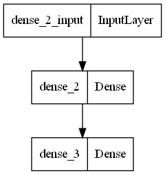
깔끔하게 확인할 수 있다. 이건 정규화 하기 전 모델이다.
정규화 한 모델 (Normalized model)

아직 조금 어려운 것 같다. . . . .
Tensorflow 는 처음이라 . . . . .
참고자료들
※ 공공빅데이터 청년인재양성 교육자료를 참고했습니다.
추가자료
+
https://koreapy.tistory.com/917
[파이썬/딥러닝] Dense Layer란? Dense Layer 역할 및 기능 / 개념
https://machinelearningknowledge.ai/keras-dense-layer-explained-for-beginners/ Keras Dense Layer Explained for Beginners - MLK - Machine Learning Knowledge In this article, we will go through tutorial of Keras Dense Layer function where will explain syntax
koreapy.tistory.com
https://underflow101.tistory.com/44
[AI 이론] Layer, 레이어의 종류와 역할, 그리고 그 이론 - 7 (Dense, Fully Connected Layer)
Dense, Fully Connected Layer 가끔 Tensorflow로 작성된 모델을 보다보면, 모델의 클래스 맨 아래쪽에 아래와 같은 코드를 볼 수 있다. # Tensorflow 2.X class SomeModel(tf.keras.Model): def __init__(self): # Some Algorithm... se
underflow101.tistory.com
https://codetorial.net/tensorflow/visualize_model.html
18. 모델 시각화하기 - Codetorial
import plot_model from keras.utils import plot_model from tensorflow.keras.utils import plot_model plot_model을 임포트할 때, tenforflow와 keras를 혼용하지 않고, 아래와 같이 사용하세요.
codetorial.net
'Data Science > Deep Learninng' 카테고리의 다른 글
| [Python/DL] 딥 러닝 (Deep Learning) - Keras (3) | 2023.01.12 |
|---|---|
| [Python/DL] 딥 러닝 (Deep Learning) (3) - 역전파(BackPropagation) (3) | 2023.01.12 |
| [Python/DL] 딥 러닝 (Deep Learning) (2) - 딥 러닝(Deep Learning) 의 학습 (3) | 2023.01.10 |
| [Python/DL] 딥 러닝 (Deep Learning) (1) - 퍼셉트론(Perceptron)과 신경망 (2) | 2023.01.10 |
| [Python/DL] 분류 알고리즘 (Classification Algorithm) : 인공신경망 (ANN : Article Neural Network) (0) | 2022.10.14 |


