
| 일 | 월 | 화 | 수 | 목 | 금 | 토 |
|---|---|---|---|---|---|---|
| 1 | 2 | 3 | ||||
| 4 | 5 | 6 | 7 | 8 | 9 | 10 |
| 11 | 12 | 13 | 14 | 15 | 16 | 17 |
| 18 | 19 | 20 | 21 | 22 | 23 | 24 |
| 25 | 26 | 27 | 28 | 29 | 30 | 31 |
- 데이터분석
- 공공빅데이터청년인턴
- decisiontree
- 공공빅데이터청년인재양성
- Keras
- 2023공공빅데이터청년인재양성
- k-means
- ML
- 머신러닝
- 분석변수처리
- 클러스터링
- 2023공빅데
- 오버샘플링
- data
- 데이터전처리
- textmining
- SQL
- ADSP
- datascience
- 빅데이터
- 2023공공빅데이터청년인재양성후기
- 공빅
- Kaggle
- ADsP3과목
- 텍스트마이닝
- DeepLearning
- 공빅데
- DL
- NLP
- machinelearning
- Today
- Total
愛林
[Data/Data Analysis] Kaggle : GTZAN Dataset - Music Genre Classification 본문
[Data/Data Analysis] Kaggle : GTZAN Dataset - Music Genre Classification
愛林 2022. 12. 21. 11:25GTZAN Dataset - Music Genre Classification
Audio Files | Mel Spectrograms | CSV with extracted features

https://www.kaggle.com/datasets/andradaolteanu/gtzan-dataset-music-genre-classification
GTZAN Dataset - Music Genre Classification
Audio Files | Mel Spectrograms | CSV with extracted features
www.kaggle.com
나는 이론보다 실전을 좋아하는 사람이다.
음성 데이터에 대해 간단하게 알아보았으니 바로 음성 데이터셋에서 유명한 GTZAN 데이터셋을
이용해서 뮤직 장르 분류를 해보려고 한다.
여기 코드를 참고해서 EDA, 전처리, 모델링까지 해보았다. (참고)
Library & Data Import
import pandas as pd
import numpy as np

import seaborn as sns
import matplotlib.pyplot as plt
%matplotlib inline

import sklearn
from sklearn.naive_bayes import GaussianNB
from sklearn.linear_model import SGDClassifier, LogisticRegression
from sklearn.neighbors import KNeighborsClassifier
from sklearn.tree import DecisionTreeClassifier
from sklearn.ensemble import RandomForestClassifier, AdaBoostClassifier
from sklearn.svm import SVC
from sklearn.neural_network import MLPClassifier
from xgboost import XGBClassifier, XGBRFClassifier
from xgboost import plot_tree, plot_importance
from sklearn.metrics import confusion_matrix, accuracy_score, roc_auc_score, roc_curve
from sklearn.decomposition import PCA
from sklearn import preprocessing
from sklearn.model_selection import train_test_split
from sklearn.feature_selection import RFE
from sklearn.metrics.pairwise import cosine_similarity

import keras
from tensorflow import keras
from keras import Sequential
from keras import layers
import tensorflow as tf
import tensorflow_addons as tfa
from tensorflow.keras.preprocessing import image_dataset_from_directory
from keras.utils.vis_utils import plot_model
from tensorflow.keras import Sequential, Input
#from keras.utils import to_categorical
from tensorflow.keras.utils import to_categorical
from tensorflow.keras.layers import Dense, Dropout,SeparableConv2D, Activation, BatchNormalization, Flatten, GlobalAveragePooling2D, Conv2D, MaxPooling2D
from tensorflow.keras.layers import Conv2D, Flatten
from tensorflow.keras.callbacks import ReduceLROnPlateau,EarlyStopping, ModelCheckpoint
from tensorflow.keras.applications.inception_v3 import InceptionV3
from tensorflow.keras.preprocessing.image import ImageDataGenerator as IDG

import librosa
import librosa.display
import IPython.display as ipd

import eli5
from eli5.sklearn import PermutationImportance

import os
import warnings
warnings.filterwarnings('ignore')
y, s = librosa.load(f'{dir_}/genres_original/blues/blues.00023.wav')

print('y:', y, '\n')
print('y shape : ', np.shape(y), '\n')
print('Sample Rate (KHz) : ', s, '\n')

print('Check Len of Audio : ', 661794/22050)
librosa 를 사용하여 블루스 악의 23번째 wav파일을 살펴보았다.
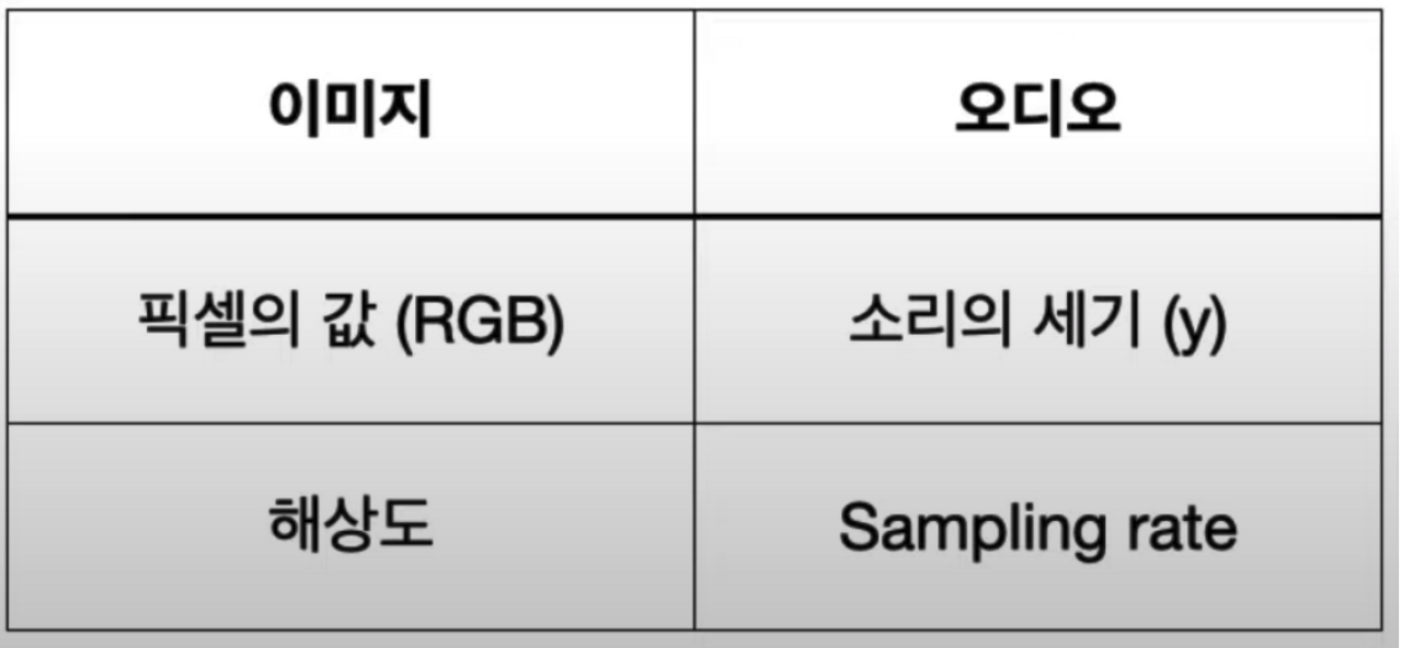
오디오 파일은 숫자로 이루어져 있다.
소리의 세기, 그리고 초당 샘플의 개수인 Sampling Rate (1초당 샘플의 개수, 1초당 Hz 또는 kHz)
위의 코드를 출력한 결과값이다.
y: [ 0.17184448  0.20730591  0.08227539 ...  0.00271606 -0.02062988
 -0.01370239]

y shape :  (661794,)

Sample Rate (KHz) :  22050

Check Len of Audio :  30.01333333333333
소리의 세기는 y, Sampling Rate 는 s이다.
y 는 661794, Sampling Rate 는 22050 kHz 이다.
음성 데이터 분석은 처음이라 큰 건지 작은 건지, 크게 의미가 없는 건지 솔직히 감을 잡기 어렵다.
audio, _ = librosa.effects.trim(y)

print('Audio File:', audio, '\n')
print('Audio File shape:', np.shape(audio))
Audio File: [ 0.17184448 0.20730591 0.08227539 ... 0.00271606 -0.02062988
-0.01370239]
Audio File shape: (661794,)librosa.effects.trim 을 이용하여 음성데이터의 선행, 후행 묵음을 제거해주었다.
안에는 소리의 세기인 y를 넣어주면 된다.
그냥 위와 같은 값이 나왔다. y가 Audio로 바뀐 것 밖에 없다.
EDA
음파 그래프를 그려보았다.
plt.figure(figsize = (16,6))
librosa.display.waveshow(y = audio, sr = s, color = '#00008B');
plt.title("Example Sound Waves On Blues", fontsize = 23)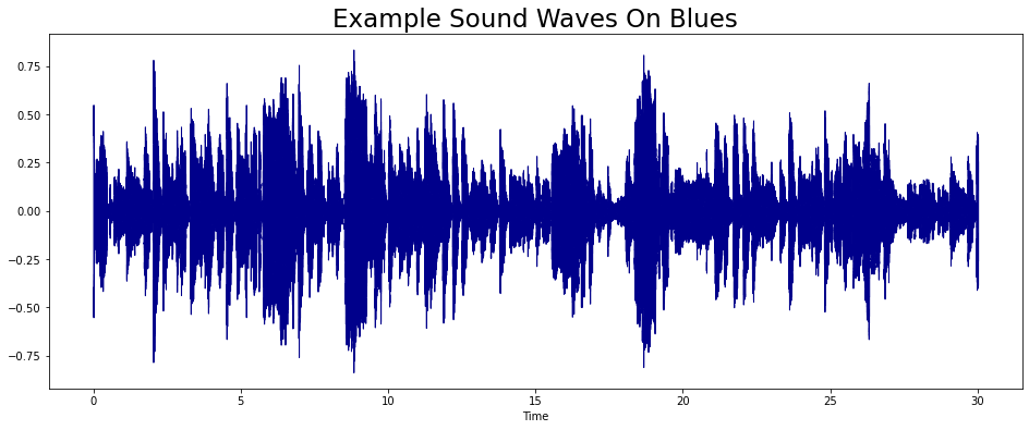
librosa.display.waveshow 를 통해서 음파를 확인할 수 있다.
이 audio 를 zero_crossings 를 이용하여 0이 되는 선을 지나친 횟수를 구해보았다.
음파가 양에서 음으로, 음에서 양으로 바뀐 비율을 뜻한다.
# Fourier Transform
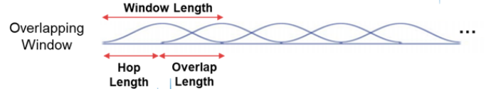
fft = 2048 # 고속 퓨리에 변환 n_fft : 음성의 길이를 어느정도로 잘라야 하는가?
hl = 512 # 교차하지 않는 길이 hop length
stft = np.abs(librosa.stft(audio, n_fft = fft, hop_length = hl)) # Short Time Fourier Transform
print(np.shape(stft))
plt.figure(figsize=(16,6))
plt.plot(stft)
plt.show()(1025, 1293)
Fourier 변환을 해주었다.
librosa.stft 를 사용하여 short time fourier transfer. 고속 퓨리에 변환을 해줄 수 있다.
파라미터 중 n_fft 는 음성의 길이를 어느 정도로 잘라서 볼 지, 앞에서 말한 Window 를 의미한다.
hop_length 는 음파 그래프에서 교차하지 않는 길이이다.
다음은 Spectogram 을 그려본다.
Spectogram 은 시간에 따른 신호 주파수의 스펙트럼 그래프이다 .
STFT 를 진행하게 되면 Spectogram이 생성되게 되는데, 이를 시각화하여 나타내보았다.
decibel = librosa.amplitude_to_db(stft ,ref = np.max) # 진폭을 데시벨로

plt.figure(figsize = (16,6))
librosa.display.specshow(decibel, sr = s, hop_length = hl, x_axis = 'time',
                        y_axis = 'log', cmap = 'cool')
plt.colorbar()
ibrosa.amplitude_to_db 를 이용하여 진폭(Amplitude) 를 데시벨(DB)로 바꾸어준다.
그리고 librosa 의 librosa.display.specshow 를 이용하여 이를 그래프로 시각화해주었다.
이것이 Spectogram이다.
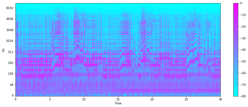
x축은 시간, y축은 데시벨(Hz) 를 나타낸다.
색깔(z축) 은 진폭을 나타낸다. 색이 진할수록 진폭이 작다는 것을 확인할 수 있다.
melspectogram 을 그려보자.
melspectogram 은 사람의 달팽이 관의 특성을 반영한 Mel-scale 을 적용한 Spectogram 표현법이다.
mel = librosa.feature.melspectrogram(audio, sr=s)
mel_db = librosa.amplitude_to_db(mel, ref = np.max)
plt.figure(figsize = (16,6))
librosa.display.specshow(mel_db, sr=s, hop_length = hl, x_axis = 'time',
                        y_axis = 'log', cmap = 'bwr')
plt.colorbar();
plt.title('Blues Mel Spectrogram', fontsize = 23)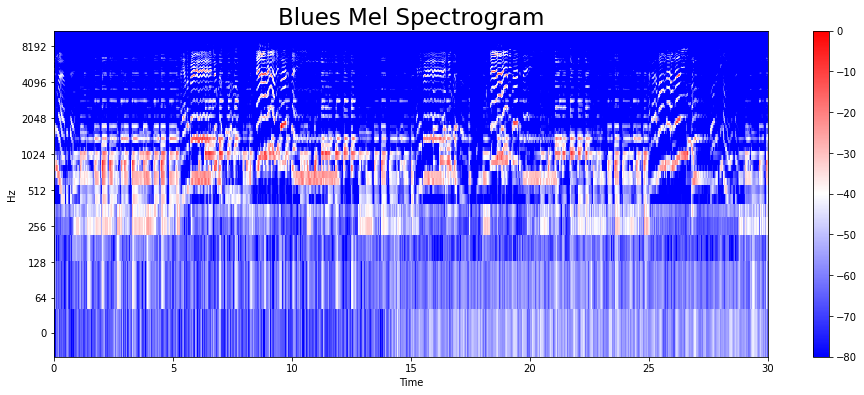
이번엔 blues 데이터가 아닌 disco 의 7번째 wav 파일을 가져와서 load 시켜주고,
Mel Spectogram 을 시각화해주었다.
y, s = librosa.load(f'{dir_}/genres_original/disco/disco.00007.wav')
y, z = librosa.effects.trim(y)

mel = librosa.feature.melspectrogram(y, sr=s)
mel_db = librosa.amplitude_to_db(mel, ref = np.max)
plt.figure(figsize = (16,6))
librosa.display.specshow(mel_db, sr=s, hop_length = hl, x_axis = 'time',
                        y_axis = 'log', cmap = 'bwr')
plt.colorbar();
plt.title('Disco Mel Spectrogram', fontsize = 23)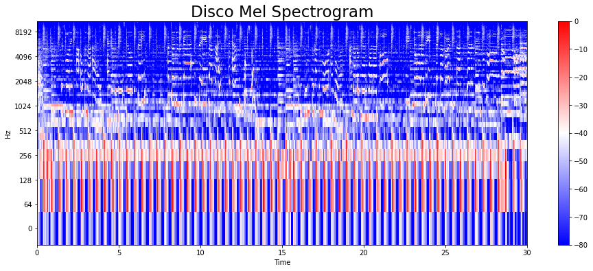
librosa.amplitude_to_db 에서 ref = np.max 파라미터가 뭔지 몰라 찾아보았다.
진폭을 데시벨(db) 로 변환하게 되면 척도가 로그가 된다.

보통 이렇게 로그 스케일로 변환시켜주는데, 이것이 plot이 될 때 우리가 듣는 것에 더 가까워진다.
데시벨 단위의 기준(dB)는 자유롭게 선택할 수 있으나, numpy.max 를 사용하면 입력이 최대값이 0db로 매핑된다.
그러면 다른 모든 값은 음수가 된다. 이 함수는 sound 범위에 대해서 임계값도 적용한다.
jazz의 15번째 파일도 동일한 프로세스로 Mel Spectogram 으로 표현해보았다.
y,s = librosa.load(f'{dir_}/genres_original/jazz/jazz.00015.wav')
y,z = librosa.effects.trim(y)

mel = librosa.feature.melspectrogram(y, sr=s)
mel_db = librosa.amplitude_to_db(mel, ref = np.max)
plt.figure(figsize= (16,6))
librosa.display.specshow(mel_db, sr=s, hop_length=hl, x_axis = 'time',
                        y_axis = 'log', cmap = 'bwr')
plt.colorbar()
plt.title("Jazz Mel Spectogram", fontsize = 23)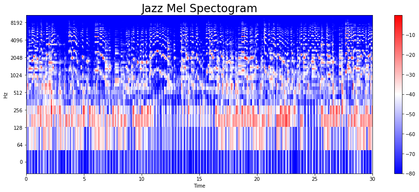
오디오 특성(Audio Feature Extraction)
을 추출해보자.
다시 blues 의 audio 파일로 돌아가서,
librosa.zero_crossings 을 이용해 0이 되는 선을 지나친 횟수인 zero cross 를 구해보자.
음파가 양에서 음으로, 음에서 양으로 바뀐 수이다.
zero_cross = librosa.zero_crossings(audio, pad = False)
print(sum(zero_cross))
# 0이 되는 선을 지나친 횟수 = 음파가 양에서 음으로, 또는 음에서 양으로 바뀐 비율3476934769번이다.
조금 더 자세히 살펴보았다.
n0 = 9000
n1 = 9040

plt.figure(figsize=(16,6))
plt.plot(y[n0:n1])
plt.grid()
plt.show()
9000에서 9040 까지를 찍어서 살펴보았다.
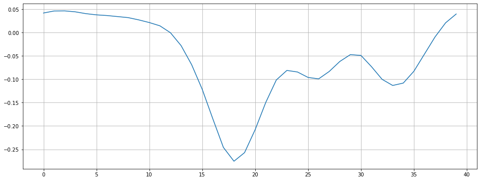
0을 지나친 횟수가 눈으로 보기엔 2번이다.
zero_crossings = librosa.zero_crossings(audio[n0:n1], pad=False) #n0 ~ n1 사이 zero crossings
print(sum(zero_crossings))2zero crossings 를 통해 살펴봐도 2개이다.
Harmonic and Percussive Components 를 구해보았다.
Harmonics 는 사람의 귀로 구분할 수 없는 특징들 (음악의 색깔) 이다.
Percussive 는 리듬과 감정을 나타내는 충격파이다.
# Harmonic and Percussive Components
# * Harmonics : 사람의 귀로 구분할 수 없는 특징들(음악의 색깔)
# * Percussives: 리듬과 감정을 나타내는 충격파

y_harm, y_perc = librosa.effects.hpss(audio)

plt.figure(figsize = (16,6))
plt.plot(y_harm, color = 'b')  # Harmonics
plt.plot(y_perc, color = 'r')   #  Percussives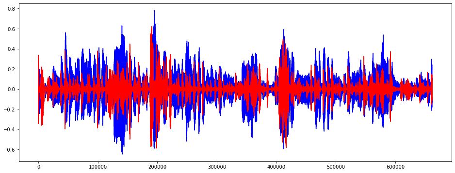
BPM 을 추출해보았다.
# 오디오 특성 추출. 템포(BPM)
tempo , _ = librosa.beat.beat_track(audio, sr = s)
tempo184.5703125음악의 빠르기인 템포이다.
성인의 건강한 심박수는 60BPM 인데.. 184라니 어느정도인지 잘 모르겠긴 하다.
그러고 보니 노래를 들어보지 않은 것 같아 들어보았다.
import IPython.display as ipd
ipd.Audio(audio, rate=s)
컨츄리 곡 느낌.
그냥 보통 정도의 빠르기인 것 같다.
소리의 무게중심을 살펴보자.
librosa.feature.spectral_centroid 를 이용했다.
소리를 주파수로 표현했을 때, 주파수의 가중평균을 계산하여 소리의 무게중심이 어디인지를 알려준다.
예를 들면, 블루스 음악은 무게 중심이 가운데에 놓여있는 반면, 메탈 음악은 보통 끝부분에서 달리기 때문에
노래의 마지막 부분에 무게중심이 실린다.
# 소리의 무게중심 살펴보기
sc = librosa.feature.spectral_centroid(audio, sr=s)[0] # 소리의 무게중심을 알려준다.

print('Centroids:', sc, '\n')
print('Shape of Spectral Centroids :', sc.shape, '\n')

frames = range(len(sc))

t = librosa.frames_to_time(frames)

print('frames:', frames, '\n')
print('t:', t)

def normalize(x, axis = 0) :
    return sklearn.preprocessing.minmax_scale(x, axis = axis)
Centroids: [1445.25434511 1363.15233037 1272.39183755 ... 937.47853521 928.49295186
913.51640189]
Shape of Spectral Centroids : (1293,)
frames: range(0, 1293)
t: [0.00000000e+00 2.32199546e-02 4.64399093e-02 ... 2.99537415e+01
2.99769615e+01 3.00001814e+01]수치로만 보면 잘 모르겠으니 시각화해서 살펴보자.
plt.figure(figsize = (16,6))
librosa.display.waveshow(audio, sr=s, alpha = 0.4, color = 'b')
plt.plot(t, normalize(sc), color = '#FFB100')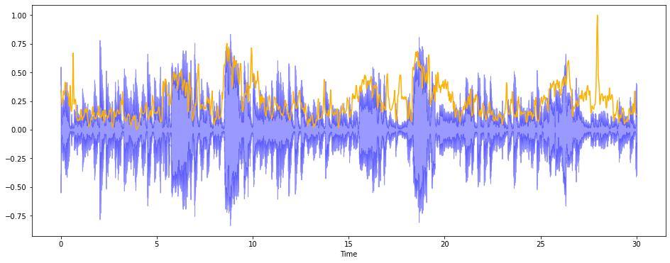
원래 곡의 wave 는 파란색으로 표시되었고,
무게중심은 노란색으로 표현했다.
librosa.feature.spectral_rolloff 를 사용하여 신호 모양을 측정했다.
총 스펙트럴 에너지 중 낮은주파수(85% 이하) 가 얼마나 많이 집중되어있는 지에 대해 시각화한 것이다.
# * 신호 모양을 측정한다.
# * 총 스펙트럴 에너지 중 낮은 주파수(85% 이하)에 얼마나 많이 집중되어 있는가
sr = librosa.feature.spectral_rolloff(audio, sr=s)[0]

# The plot
plt.figure(figsize = (16,6))
librosa.display.waveshow(audio, sr=s, alpha = 0.4, color = 'b')
plt.plot(t, normalize(sr),color = 'r')
이제 Feature 를 보기 위한 MFCC(Mel Frequency Cepstral Coefficient) 를 해보자.
MFCC는 소리의 대표적인 특성이라고 이해할 수 있겠다.
Mel scale 을 쓰기 때문에 사람의 청각 특성에 맞추어져 있다.
# MFCC
mfcc = librosa.feature.mfcc(audio, sr=s)
print(mfcc.shape)

plt.figure(figsize= (16,6))
librosa.display.specshow(mfcc, sr=s, x_axis='time', cmap = 'cool')
(20, 1293)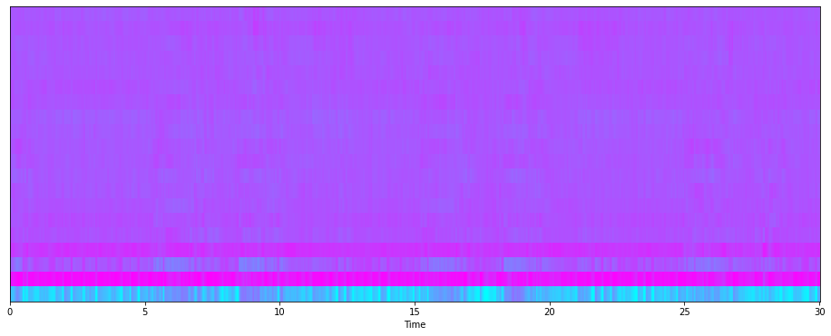
mfcc 한 결과를 scaling 하고 살펴보았다.
평균과 분산까지 도출해냈다.
mfcc = sklearn.preprocessing.scale(mfcc, axis = 1)
print('Mean :', mfcc.mean(), '\n')
print('Var :', mfcc.var())

plt.figure(figsize=  (16,6))
librosa.display.specshow(mfcc, sr=s, x_axis = 'time', cmap = 'bwr');
Mean : 1.1801075e-09
Var : 1.0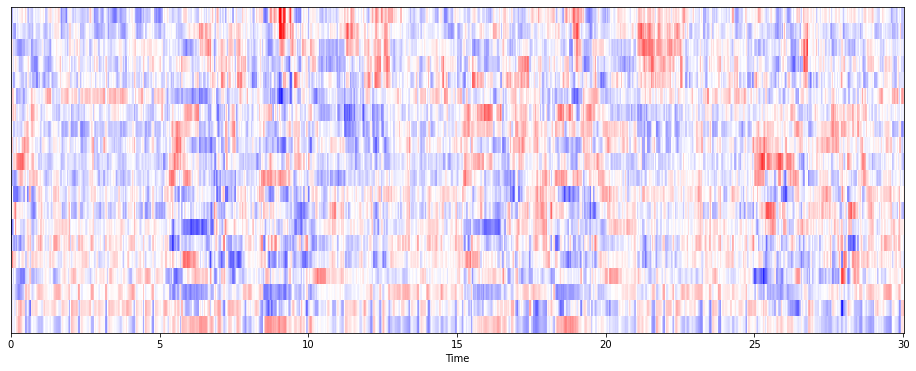
Chroma Fequencies . 크로마 특징을 살펴보았다.
크로마 특징은 음악의 강렬한 표현으로, 인간 청각이 옥타브 차이가 나는 주파수를 가진 두 음을 유사음으로
인지한다는 음악이론에 기반한다.
그러므로, 화음 인식에 좋다.
모든 스펙트럼을 12개의 Bin으로 표현한다.
C,C#,D,D#,E,F,F#,G,G#,A,A#,B 의 Pitch Class 를 갖는다.
hl = 5000

#
chromagram = librosa.feature.chroma_stft(audio, sr=s, hop_length = hl)
print('Chromagram shape:', chromagram.shape)

plt.figure(figsize = (16,6))
librosa.display.specshow(chromagram, x_axis = 'time', y_axis = 'chroma', hop_length = hl,
                        cmap = 'bwr')
Chromagram shape: (12, 133)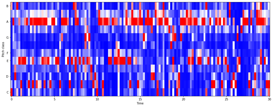
이렇게 EDA로 살펴본 특징들을 학습시켜 음악장르 분류 알고리즘을 만들어보자.
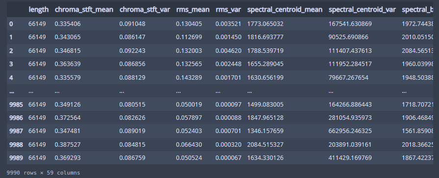
df = pd.read_csv(f'{dir_}/features_30_sec.csv')
이미 feature 가 다 csv파일로 나와있어서 사실 그냥 분류 모델에 때려넣기만 하면 된다 ..
60개의 column과 1000개의 row 를 가졌다.
np.ones_like 는 주어진 형태와 타입을 갖는 1로 채워진 어레이를 반환합니다. 이로 상삼각행렬을 만들어준 뒤,
삼각 상관관계 그래프를 시각화했다.
spike = [col for col in df.columns if 'mean' in col]
corr =  df[spike].corr()

mask = np.triu(np.ones_like(corr, dtype = np.bool))

f, ax=  plt.subplots(figsize = (16,11))

sns.heatmap(corr, mask=mask, cmap = 'bwr', vmax =.3, center = 0,
           square = True, linewidths = .5, cbar_kws = {'shrink' : .5})

plt.xticks(fontsize = 10)
plt.yticks(fontsize = 10)
mfcc2_mean 과 다른 feature 들이 꽤나 높은 상관관계가 있는 것을 확인했다.
x = df[['label', 'tempo']]

f, ax=  plt.subplots(figsize = (16,9))
sns.boxplot(x = 'label', y='tempo', data =x, palette = 'summer')

plt.title('BPM Boxplot for Genres', fontsize = 25)
plt.xticks(fontsize = 14)
plt.yticks(fontsize = 10)
plt.xlabel('Genre', fontsize = 15)
plt.ylabel('BPM', fontsize = 15)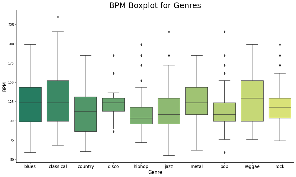
장르에 따른 BPM 을 boxplot 으로 시각화해주었다.
hiphop 과 pop 은 역시 엄청 빠른 곡도 있고 느린 곡도 있어서 이상치가 꽤나 크다.
아까 우리가 들은 Blues 곡은 평균에 비해 빠른 편이었던 것 같다.
Scaling
modeling 을 진행하기전, scaling 을 먼저 진행해주었다.
df = df.iloc[0:, 1:]
y = df['label']
X = df.loc[:, df.columns != 'label']

cols = X.columns
scaler = preprocessing.MinMaxScaler()
np_scaled = scaler.fit_transform(X)
X = pd.DataFrame(np_scaled, columns = cols)

pca = PCA(n_components = 2)
scaled_df = pca.fit_transform(X)
df_p = pd.DataFrame(data = scaled_df, columns = ['pca1', 'pca2'])

fdf = pd.concat([df_p, y], axis = 1)

pca.explained_variance_ratio_
array([0.24644968, 0.22028192])target 데이터와 x데이터를 나누어주고,
x 데이터들은 MinMaxScaler 를 통해서 scaling 해주었다.
이후 pca 를 통해 2차원로 차원축소를 진행한 뒤, pca dataframe 을 만들어주었다.
이후 pca한 결과와 Target 데이터를 결합시켰다.
explained_variance_ratio_ 를 구해보니 PCA 결과가 딱히 데이터를 크게 설명하는 것 같아 보이지 않는다 ..
2차원으로 차원축소 한 김에 시각화해주었다.
plt.figure(figsize= (16,9))
sns.scatterplot(x = 'pca1', y = 'pca2', data = fdf, hue = 'label', alpha = 0.7,
               s = 100)

plt.title('Genres with PCA', fontsize = 25)
plt.xticks(fontsize = 14)
plt.yticks(fontsize = 10)
plt.xlabel("Principal Components 1", fontsize = 15)
plt.ylabel("Principal Components 2", fontsize = 15)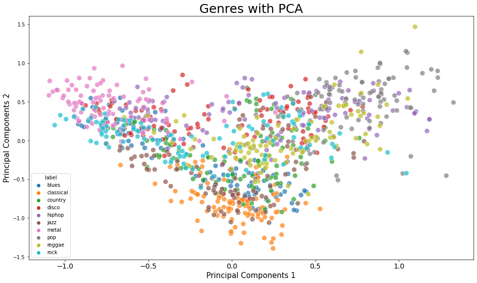
중구난방이다.
modeling 을 진행해보자.
Modeling
df = pd.read_csv(f'{dir_}/features_3_sec.csv')
df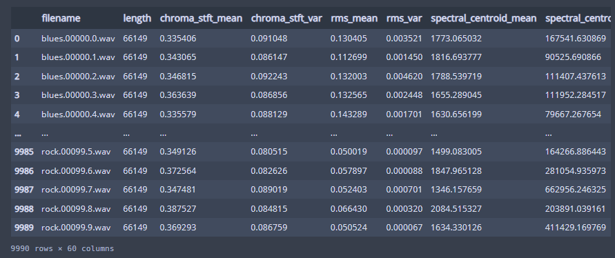
3초 feature 을 불러왔다.
df = df.iloc[0:,1:]
df
file name 은 필요없는 column 같아 보이니 없애준다.
y = df['label']
X = df.loc[:, df.columns != 'label']

cols = X.columns
scaler = preprocessing.MinMaxScaler()
np_scaled = scaler.fit_transform(X)

X = pd.DataFrame(np_scaled, columns = cols)
마찬가지로 x, y(Target) 을 분리시켜주고,
MinMaxScaler 를 통해 scaling 시켜준다.
X_train, X_test, y_train, y_test = train_test_split(X, y, test_size = 0.3, random_state= 42)train 데이터와 test 데이터셋을 분리시켜주고,
def model_assess(model, title = 'Default') :
    model.fit(X_train, y_train)
    preds = model.predict(X_test)
    print(confusion_matrix(y_test, preds))
    print('Accuracy ', title, ':', round(accuracy_score(y_test, preds), 5), '\n')
모델을 적용하기 전 모델을 적용하고 accuracy score를 내주는 함수를 만들어주었다.
nb = GaussianNB()
model_assess(nb, "Naive Bayes")

sgd = SGDClassifier()
model_assess(sgd, "Stochastic Gradient Descent")

knn = KNeighborsClassifier(n_neighbors = 19)
model_assess(knn, 'KNN')

tree = DecisionTreeClassifier()
model_assess(tree, 'Decision Trees')

rf = RandomForestClassifier(n_estimators = 1000, max_depth = 10, random_state = 0)
model_assess(rf, 'Random Forest')

svm = SVC(decision_function_shape = 'ovo')
model_assess(svm, "Support Vector Machine")

lg = LogisticRegression(random_state = 0, solver = 'lbfgs', multi_class = 'multinomial')
model_assess(lg, 'Logistic Regression')

mlp = MLPClassifier(solver = 'lbfgs', alpha = 1e-5, hidden_layer_sizes= (5000,10),
                   random_state= 1)
model_assess(mlp, "Neural Nets")

ada = AdaBoostClassifier(n_estimators = 1000)
model_assess(ada, 'AdaBoost')
[[100 6 61 12 1 19 85 0 12 23]
[ 0 275 1 0 0 21 0 0 1 10]
[ 20 11 166 25 4 8 22 11 10 9]
[ 13 4 30 102 13 2 57 46 17 17]
[ 8 1 15 36 109 0 44 60 36 2]
[ 10 59 34 6 0 117 8 13 5 34]
[ 5 0 3 11 3 0 269 0 3 9]
[ 0 0 17 18 2 1 0 208 13 8]
[ 19 1 61 10 23 3 6 29 149 15]
[ 8 6 49 40 2 7 96 13 17 62]]
Accuracy Naive Bayes : 0.51952
[[187 1 0 0 4 31 54 0 3 39]
[ 2 275 0 0 0 23 0 0 0 8]
[ 30 0 56 1 5 55 8 18 3 110]
[ 3 3 1 56 38 18 38 55 2 87]
[ 4 2 4 1 209 4 37 31 3 16]
[ 11 17 1 0 0 244 0 4 4 5]
[ 5 0 0 0 4 1 285 0 0 8]
[ 0 0 0 0 3 5 0 245 1 13]
[ 12 2 0 7 63 17 19 26 121 49]
[ 16 2 2 2 7 35 48 21 6 161]]
Accuracy Stochastic Gradient Descent : 0.61361
[[256 5 22 4 2 8 6 0 10 6]
[ 0 297 1 0 0 10 0 0 0 0]
[ 9 2 230 11 1 13 0 1 12 7]
[ 7 6 8 246 8 0 2 4 6 14]
[ 7 1 15 24 217 0 9 21 14 3]
[ 2 30 16 2 0 233 0 2 1 0]
[ 6 0 2 15 5 0 252 0 4 19]
[ 0 0 6 17 2 2 0 229 10 1]
[ 3 1 16 20 13 0 2 11 248 2]
[ 11 1 20 35 0 7 7 2 10 207]]
Accuracy KNN : 0.80581
[[163 3 38 18 16 15 13 6 19 28]
[ 5 261 10 1 0 23 0 1 1 6]
[ 29 8 146 11 11 19 9 8 14 31]
[ 11 1 13 158 30 7 7 24 11 39]
[ 7 1 11 32 205 4 11 17 20 3]
[ 17 16 13 7 2 209 2 9 1 10]
[ 13 0 6 13 8 3 236 2 5 17]
[ 0 1 13 13 13 5 1 204 7 10]
[ 12 2 16 20 27 5 5 16 193 20]
[ 18 5 27 26 13 21 25 6 13 146]]
Accuracy Decision Trees : 0.64097
[[246 1 31 8 4 8 15 0 6 0]
[ 0 294 1 0 0 12 0 0 0 1]
[ 13 1 212 12 0 23 3 3 9 10]
[ 1 4 11 235 14 1 5 8 10 12]
[ 4 0 7 8 250 2 13 15 10 2]
[ 7 21 5 1 0 251 0 0 1 0]
[ 1 0 1 2 3 1 281 0 6 8]
[ 0 0 12 4 2 1 0 238 5 5]
[ 5 2 9 11 7 4 4 17 254 3]
[ 7 2 29 34 1 12 19 4 13 179]]
Accuracy Random Forest : 0.81415
[[241 5 10 9 2 12 24 0 7 9]
[ 0 294 2 0 0 10 0 0 0 2]
[ 19 0 192 18 0 23 1 5 5 23]
[ 2 6 7 199 18 7 10 12 14 26]
[ 7 2 7 18 220 0 8 16 28 5]
[ 12 25 9 2 0 234 0 1 2 1]
[ 10 0 0 7 4 0 270 0 2 10]
[ 0 1 10 8 4 1 0 233 4 6]
[ 13 2 16 18 20 3 5 10 220 9]
[ 19 2 24 45 7 11 16 9 10 157]]
Accuracy Support Vector Machine : 0.75409
[[212 5 12 7 4 18 40 0 11 10]
[ 2 287 5 0 0 10 0 0 0 4]
[ 23 1 166 18 2 21 1 19 9 26]
[ 3 5 15 182 23 3 16 21 15 18]
[ 8 2 8 17 201 0 15 24 31 5]
[ 11 28 14 5 1 214 0 2 7 4]
[ 10 0 0 7 4 0 266 0 3 13]
[ 0 0 14 8 11 0 0 226 3 5]
[ 14 1 19 12 29 5 8 10 210 8]
[ 35 3 25 32 5 14 22 18 19 127]]
Accuracy Logistic Regression : 0.6977
[[192 2 52 2 4 17 21 0 16 13]
[ 2 287 2 1 0 15 0 0 1 0]
[ 20 1 152 11 1 32 0 4 17 48]
[ 2 4 7 165 30 3 11 18 17 44]
[ 6 0 3 22 203 3 10 27 31 6]
[ 9 32 19 0 0 207 1 2 4 12]
[ 15 0 1 6 6 0 261 0 0 14]
[ 0 0 1 8 4 0 0 235 13 6]
[ 5 1 23 23 27 1 3 16 216 1]
[ 22 2 46 48 2 15 19 9 13 124]]
Accuracy Neural Nets : 0.68135
[[110 2 23 17 7 10 122 0 19 9]
[ 3 283 2 1 1 12 0 0 1 5]
[ 49 8 79 10 36 10 18 35 21 20]
[ 11 7 6 77 23 0 58 86 19 14]
[ 8 3 7 37 73 1 93 65 20 4]
[ 29 60 16 14 11 92 11 27 13 13]
[ 4 0 2 5 3 0 283 0 0 6]
[ 0 1 6 5 6 0 0 242 6 1]
[ 25 5 25 30 40 0 22 60 103 6]
[ 31 4 23 42 10 6 72 55 12 45]]
Accuracy AdaBoost : 0.4628 RandomForest 모델이 가장 높은 accuracy 를 보여주고 있다.
이 분류기를 통하여 분리시켜둔 test 데이터를 predict 해보자.
이후 정확도 검증을 위해 Confusion_Matrix 를 시각화하여 확인했다.
rf = RandomForestClassifier(n_estimators = 1000, max_depth = 10, random_state= 0)
rf.fit(X_train, y_train)

preds =  rf.predict(X_test)

print('Accuracy', ':', round(accuracy_score(y_test, preds), 5), '\n')

conf = confusion_matrix(y_test, preds)

plt.figure(figsize = (16,9))
sns.heatmap(conf, cmap = 'bwr', annot = True,
           xticklabels = ["blues", "classical", "country", "disco", "hiphop",
                          "jazz", "metal", "pop", "reggae", "rock"],
           yticklabels=["blues", "classical", "country", "disco", "hiphop",
                        "jazz", "metal", "pop", "reggae", "rock"])
Accuracy : 0.81415 
대충 어느정도 잘 분류해내고 있는 것 같다.
아쉽긴 하지만 ..
변수중요도를 살펴보았다.
# 변수 중요도 결정
perm = PermutationImportance(estimator=rf, random_state=1)
perm.fit(X_test, y_test)

eli5.show_weights(estimator=perm, feature_names = X_test.columns.tolist())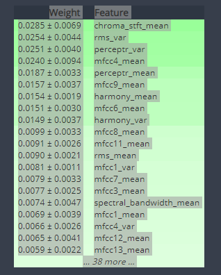
Finding Similar Song
위와 같은 분류를 바탕으로,
내가 선택한 노래와 유사도가 높은 노래를 찾아주는 시스템을 만들어보자.
df = pd.read_csv(f'{dir_}/features_30_sec.csv', index_col='filename')

labels = df[['label']]

df = df.drop(columns=['length','label'])
df

scaled=preprocessing.scale(df)
print('Scaled data type:', type(scaled))
데이터를 로드시켜주고, length 와 label은 빼주었다.
이후 스케일링까지 진행했다.
similarity = cosine_similarity(scaled)
print("Similarity shape:", similarity.shape)
sim_df_labels = pd.DataFrame(similarity)
sim_df_names = sim_df_labels.set_index(labels.index)
sim_df_names.columns = labels.index

sim_df_names.head()
코사인 유사도 (cosine_similarity) 를 사용했다.
코사인유사도는 벡터간 각도를 통한 유사도인데, 1에 가까울수록 유사하고 -1에 가까울수록 유사하지 않다.

비슷한 노래를 찾아주는 함수를 만들어주었다.
def find_similar_songs(name):
    series = sim_df_names[name].sort_values(ascending = False)
    series = series.drop(name)
    print("\n*******\nSimilar songs to ", name)
    print(series.head(5))
find_similar_songs('rock.00011.wav')
ipd.Audio(f'{dir_}/genres_original/rock/rock.00011.wav')rock 의 11번 wav와 유사한 노래들을 뽑아보았다.
*******
Similar songs to  rock.00011.wav
filename
country.00054.wav    0.600560
jazz.00095.wav       0.593636
jazz.00027.wav       0.554560
jazz.00038.wav       0.544000
jazz.00015.wav       0.530824
Name: rock.00011.wav, dtype: float64
rock 음악을 넣었는데 contry 54, jazz 95, jazz27, jazz38, jazz15 가 나왔다.
rock인데 웬 country랑 jazz? 했는데 rock 주제에 country 스러웠다.
해당 음악들을 찾아서 확인해보았다.
ipd.Audio(f'{dir_}/genres_original/country/country.00054.wav')ipd.Audio(f'{dir_}/genres_original/jazz/jazz.00095.wav')유사한 지 잘 모르겠으나, 내 음악취향이 아니라서 그런 걸수도 있다.
jazz95번은 나름 맘에 드는 듯.
Youtube 뮤직 알고리즘이 내 스타일 노래를 척척 잘 찾아주던데,
이런 기반이겠다는 생각을 했다.
현재 나와있는 가요들로 해봐도 재밌을 것 같다.
참고
https://www.kaggle.com/code/praveen14/audio-data-eda-processing-modeling-recommend
Audio Data: EDA, Processing, Modeling & Recommend
Explore and run machine learning code with Kaggle Notebooks | Using data from GTZAN Dataset - Music Genre Classification
www.kaggle.com
https://jonhyuk0922.tistory.com/114
[Librosa] 음성인식 기초 및 음악분류 & 추천 알고리즘
https://link.coupang.com/a/sJVpO Apple 아이패드 10.2 2021년 9세대 COUPANG www.coupang.com 안녕하세요~ 27년차 진로탐색꾼 조녁입니다!! 오늘은 음성파일을 인식하고 거기서 특징추출하는 기초적인 내용부터 추
jonhyuk0922.tistory.com
위의 코드와 알고리즘 함수들을 사용할 때 해당 블로그를 참고.


