
| 일 | 월 | 화 | 수 | 목 | 금 | 토 |
|---|---|---|---|---|---|---|
| 1 | 2 | 3 | ||||
| 4 | 5 | 6 | 7 | 8 | 9 | 10 |
| 11 | 12 | 13 | 14 | 15 | 16 | 17 |
| 18 | 19 | 20 | 21 | 22 | 23 | 24 |
| 25 | 26 | 27 | 28 | 29 | 30 | 31 |
- 데이터전처리
- ML
- 공빅데
- 데이터분석
- SQL
- 2023공공빅데이터청년인재양성
- ADSP
- 빅데이터
- k-means
- 2023공공빅데이터청년인재양성후기
- 텍스트마이닝
- 오버샘플링
- 공빅
- decisiontree
- machinelearning
- datascience
- textmining
- 공공빅데이터청년인턴
- Keras
- NLP
- 2023공빅데
- Kaggle
- 분석변수처리
- 머신러닝
- 공공빅데이터청년인재양성
- DeepLearning
- 클러스터링
- data
- DL
- ADsP3과목
- Today
- Total
愛林
[Data/Data Analysis] Kaggle : 주택 가격 예측 모델 만들기 (House Prices: Advanced Regression Techniques) - (1) 본문
[Data/Data Analysis] Kaggle : 주택 가격 예측 모델 만들기 (House Prices: Advanced Regression Techniques) - (1)
愛林 2022. 9. 30. 14:50House Prices Data Analysis

www.kaggle.com/c/house-prices-advanced-regression-techniques
House Prices - Advanced Regression Techniques | Kaggle
www.kaggle.com
너무나도 유명한 House Prices Data 를 분석해보자.
내가 알기로는 Scikit Learn에서 제공하는 load 데이터에 보스턴 주택 가격 데이터가
있었던 걸로 알고 있는데, 그게 이 데이터랑 같은 지는 잘 모르겠다.
이번에도 다른 사람들의 코드를 참고하여 거의 필사 수준의 코딩을 했다.
나도 데이터분석 잘하고 싶어.
이 Competition 의 목적은 주어진 데이터로 집값을 예측하는 것이다.
데이터를 통해 각 요소들이 집값에 주는 영향을 살펴보고,
그 요소들을 통해서 집값을 예측해볼 것이다.
데이터 살펴보기
분석에 들어가기 전, 먼저 Data Dictionary 를 살펴보고 어떤 데이터들이 있는 지 파악해보자.
믿을 수 없지만 여기 데이터는 무려 칼럼이 81개이다.
Data Dictionary
- SalePrice - 부동산의 판매 가격(달러)입니다. 이것은 예측하려는 대상 변수입니다.
- MSSubClass : 건물 클래스
- MSZoning : 일반 구역 분류
- LotFrontage : 부동산에 연결된 거리의 선형 피트
- LotArea : 평방 피트 단위의 부지 크기
- Street : 도로 접근 유형
- Alley : 골목 접근 방식
- LotShape : 속성의 일반적인 모양
- LandContour : 부동산의 평탄도
- Utilities : 사용 가능한 유틸리티 유형
- LotConfig : 로트 구성
- LandSlope : 속성의 기울기
- Neighborhood : Ames 시 경계 내의 물리적 위치
- Condition1 : 간선도로 또는 철도와 인접
- Condition2 : 간선도로 또는 철도와의 근접성(초가 있는 경우)
- BldgType : 주거 유형
- HouseStyle : 주거 스타일
- OverallQual : 전체재질 및 마감품질
- OverallCond : 전체 상태 등급
- YearBuilt : 원래 건설 날짜
- YearRemodAdd : 리모델링 날짜
- RoofStyle : 지붕 유형
- RoofMatl : 지붕 재료
- ExterQual1st : 주택의 외부 피복
- ExterQual2nd : 주택의 외부 덮음(하나 이상의 재료인 경우)
- MasVnrType : 석조 베니어 유형
- MasVnrArea : 석조 베니어판 면적(제곱피트)
- ExterQual : 외장재 품질
- ExterCond : 외장재의 현황
- Foundation : 기반의 종류
- BsmtQual : 지하실 높이
- BsmtCond : 지하실의 일반 상태
- BsmtExposure : 파업 또는 정원 수준의 지하 벽
- BsmtFinType1 : 지하실 마감 면적의 품질
- BsmtFinSF1 : 1종 제곱피트 완성
- BsmtFinType2 : 두 번째 완성 영역의 품질(있는 경우)
- BsmtFinSF2 : 유형 2 완성 평방 피트
- BsmtUnfSF : 지하실의 미완성 평방 피트
- TotalBsmtSF : 지하실의 총 평방 피트
- Heating : 난방의 종류
- HeatingQC : 난방 품질 및 상태
- CentralAir : 중앙 에어컨
- Electrical : 전기 시스템
- 1stFlrSF : 1층 평방피트
- 2ndFlrSF : 2층 평방피트
- LowQualFinSF : 저품질 마감 평방 피트(모든 층)
- GrLivArea : 지상(지상) 거실 면적 평방피트
- BsmtFullBath : 지하 전체 욕실
- BsmtHalfBath : 지하 반 화장실
- FullBath : 등급 이상의 전체 욕실
- HalfBath : 등급 이상의 반욕
- Bedroom : 지하층 이상의 침실 수
- kitchen : 주방 수
- KitchenQual : 주방 품질
- TotRmsAbvGrd : 등급 이상의 총 방(화장실 제외)
- Functional : 홈 기능 등급
- Fireplaces : 벽난로의 수
- FireplaceQu : 벽난로 품질
- GarageType : 차고 위치
- GarageYrBlt : 차고 건설 연도
- GarageFinish : 차고 인테리어 마감
- GarageCars : 차고의 차고 크기
- GarageArea : 평방 피트의 차고 크기
- GarageQual : 차고 품질
- GarageCond : 차고 상태
- PavedDrive : 포장된 차도
- WoodDeckSF : 평방 피트의 목재 데크 면적
- OpenPorchSF : 평방 피트의 오픈 베란다 영역
- EnclosedPorch : 평방 피트의 닫힌 베란다 영역
- 3SsnPorch : 제곱피트의 3계절 베란다 면적
- ScreenPorch : 평방 피트의 스크린 베란다 면적
- PoolArea : 평방 피트의 수영장 면적
- PoolQC : 수영장 품질
- Fence : 울타리 품질
- MiscFeature : 다른 범주에서 다루지 않는 기타 기능
- MiscVal : 기타 기능의 $값
- MoSold : 월 판매
- YrSold : 판매 연도
- SaleType : 판매유형
- SaleCondition : 판매조건
먼저 필요한 라이브러리들을 import 해주고 train, test 데이터를 불러왔다.
import numpy as np
import pandas as pd
import matplotlib.pyplot as plt
import seaborn as sns
plt.style.use('fivethirtyeight')
import warnings
warnings.filterwarnings('ignore')
%matplotlib inline
train = pd.read_csv('train.csv')
test = pd.read_csv('test.csv')train.head()
test.head()
train.columnsIndex(['Id', 'MSSubClass', 'MSZoning', 'LotFrontage', 'LotArea', 'Street',
'Alley', 'LotShape', 'LandContour', 'Utilities', 'LotConfig',
'LandSlope', 'Neighborhood', 'Condition1', 'Condition2', 'BldgType',
'HouseStyle', 'OverallQual', 'OverallCond', 'YearBuilt', 'YearRemodAdd',
'RoofStyle', 'RoofMatl', 'Exterior1st', 'Exterior2nd', 'MasVnrType',
'MasVnrArea', 'ExterQual', 'ExterCond', 'Foundation', 'BsmtQual',
'BsmtCond', 'BsmtExposure', 'BsmtFinType1', 'BsmtFinSF1',
'BsmtFinType2', 'BsmtFinSF2', 'BsmtUnfSF', 'TotalBsmtSF', 'Heating',
'HeatingQC', 'CentralAir', 'Electrical', '1stFlrSF', '2ndFlrSF',
'LowQualFinSF', 'GrLivArea', 'BsmtFullBath', 'BsmtHalfBath', 'FullBath',
'HalfBath', 'BedroomAbvGr', 'KitchenAbvGr', 'KitchenQual',
'TotRmsAbvGrd', 'Functional', 'Fireplaces', 'FireplaceQu', 'GarageType',
'GarageYrBlt', 'GarageFinish', 'GarageCars', 'GarageArea', 'GarageQual',
'GarageCond', 'PavedDrive', 'WoodDeckSF', 'OpenPorchSF',
'EnclosedPorch', '3SsnPorch', 'ScreenPorch', 'PoolArea', 'PoolQC',
'Fence', 'MiscFeature', 'MiscVal', 'MoSold', 'YrSold', 'SaleType',
'SaleCondition', 'SalePrice'],
dtype='object')칼럼 너무 많아 ~
train.info()<class 'pandas.core.frame.DataFrame'>
RangeIndex: 1460 entries, 0 to 1459
Data columns (total 81 columns):
# Column Non-Null Count Dtype
--- ------ -------------- -----
0 Id 1460 non-null int64
1 MSSubClass 1460 non-null int64
2 MSZoning 1460 non-null object
3 LotFrontage 1201 non-null float64
4 LotArea 1460 non-null int64
5 Street 1460 non-null object
6 Alley 91 non-null object
7 LotShape 1460 non-null object
8 LandContour 1460 non-null object
9 Utilities 1460 non-null object
10 LotConfig 1460 non-null object
11 LandSlope 1460 non-null object
12 Neighborhood 1460 non-null object
13 Condition1 1460 non-null object
14 Condition2 1460 non-null object
15 BldgType 1460 non-null object
16 HouseStyle 1460 non-null object
17 OverallQual 1460 non-null int64
18 OverallCond 1460 non-null int64
19 YearBuilt 1460 non-null int64
20 YearRemodAdd 1460 non-null int64
21 RoofStyle 1460 non-null object
22 RoofMatl 1460 non-null object
23 Exterior1st 1460 non-null object
24 Exterior2nd 1460 non-null object
25 MasVnrType 1452 non-null object
26 MasVnrArea 1452 non-null float64
27 ExterQual 1460 non-null object
28 ExterCond 1460 non-null object
29 Foundation 1460 non-null object
30 BsmtQual 1423 non-null object
31 BsmtCond 1423 non-null object
32 BsmtExposure 1422 non-null object
33 BsmtFinType1 1423 non-null object
34 BsmtFinSF1 1460 non-null int64
35 BsmtFinType2 1422 non-null object
36 BsmtFinSF2 1460 non-null int64
37 BsmtUnfSF 1460 non-null int64
38 TotalBsmtSF 1460 non-null int64
39 Heating 1460 non-null object
40 HeatingQC 1460 non-null object
41 CentralAir 1460 non-null object
42 Electrical 1459 non-null object
43 1stFlrSF 1460 non-null int64
44 2ndFlrSF 1460 non-null int64
45 LowQualFinSF 1460 non-null int64
46 GrLivArea 1460 non-null int64
47 BsmtFullBath 1460 non-null int64
48 BsmtHalfBath 1460 non-null int64
49 FullBath 1460 non-null int64
50 HalfBath 1460 non-null int64
51 BedroomAbvGr 1460 non-null int64
52 KitchenAbvGr 1460 non-null int64
53 KitchenQual 1460 non-null object
54 TotRmsAbvGrd 1460 non-null int64
55 Functional 1460 non-null object
56 Fireplaces 1460 non-null int64
57 FireplaceQu 770 non-null object
58 GarageType 1379 non-null object
59 GarageYrBlt 1379 non-null float64
60 GarageFinish 1379 non-null object
61 GarageCars 1460 non-null int64
62 GarageArea 1460 non-null int64
63 GarageQual 1379 non-null object
64 GarageCond 1379 non-null object
65 PavedDrive 1460 non-null object
66 WoodDeckSF 1460 non-null int64
67 OpenPorchSF 1460 non-null int64
68 EnclosedPorch 1460 non-null int64
69 3SsnPorch 1460 non-null int64
70 ScreenPorch 1460 non-null int64
71 PoolArea 1460 non-null int64
72 PoolQC 7 non-null object
73 Fence 281 non-null object
74 MiscFeature 54 non-null object
75 MiscVal 1460 non-null int64
76 MoSold 1460 non-null int64
77 YrSold 1460 non-null int64
78 SaleType 1460 non-null object
79 SaleCondition 1460 non-null object
80 SalePrice 1460 non-null int64
dtypes: float64(3), int64(35), object(43)
memory usage: 924.0+ KB눈에 띄게 Null 값이 많은 칼럼들이 보인다. 심지어 Object 타입이야.
얘네는 나중에 제거해주어야 겠다는 생각이 든다.
load_Boston Dataset 과는 다른 데이터인 것 같다. 변수가 다르네
EDA (탐색적 데이터 분석) 진행
EDA(탐색적 데이터 분석) 을 통해 데이터의 특징에 대해 좀 더 세부적으로 알아보자.
데이터의 문제점이나 패턴 등을 파악하고 이후 전처리를 어떻게 할 지에 대해서 구체화시킨다.
변수가 너무 많기 때문에 Numerical 변수와 Categorical 변수를 나누어서 살펴보자.
1. 변수
numerical_feats = train.dtypes[train.dtypes != "object"].index
print("Number of Numerical features: ", len(numerical_feats))

categorical_feats = train.dtypes[train.dtypes == "object"].index
print("Number of Categorical features: ", len(categorical_feats))
Number of Numerical features: 38
Number of Categorical features: 43Numerical 변수는 38개, Categorical 변수는 43개이다.
print(train[numerical_feats].columns)
print("*"*80)
print(train[categorical_feats].columns)
Index(['Id', 'MSSubClass', 'LotFrontage', 'LotArea', 'OverallQual',
'OverallCond', 'YearBuilt', 'YearRemodAdd', 'MasVnrArea', 'BsmtFinSF1',
'BsmtFinSF2', 'BsmtUnfSF', 'TotalBsmtSF', '1stFlrSF', '2ndFlrSF',
'LowQualFinSF', 'GrLivArea', 'BsmtFullBath', 'BsmtHalfBath', 'FullBath',
'HalfBath', 'BedroomAbvGr', 'KitchenAbvGr', 'TotRmsAbvGrd',
'Fireplaces', 'GarageYrBlt', 'GarageCars', 'GarageArea', 'WoodDeckSF',
'OpenPorchSF', 'EnclosedPorch', '3SsnPorch', 'ScreenPorch', 'PoolArea',
'MiscVal', 'MoSold', 'YrSold', 'SalePrice'],
dtype='object')
********************************************************************************
Index(['MSZoning', 'Street', 'Alley', 'LotShape', 'LandContour', 'Utilities',
'LotConfig', 'LandSlope', 'Neighborhood', 'Condition1', 'Condition2',
'BldgType', 'HouseStyle', 'RoofStyle', 'RoofMatl', 'Exterior1st',
'Exterior2nd', 'MasVnrType', 'ExterQual', 'ExterCond', 'Foundation',
'BsmtQual', 'BsmtCond', 'BsmtExposure', 'BsmtFinType1', 'BsmtFinType2',
'Heating', 'HeatingQC', 'CentralAir', 'Electrical', 'KitchenQual',
'Functional', 'FireplaceQu', 'GarageType', 'GarageFinish', 'GarageQual',
'GarageCond', 'PavedDrive', 'PoolQC', 'Fence', 'MiscFeature',
'SaleType', 'SaleCondition'],
dtype='object')변수명을 추출해보았다.
2. 이상값 확인
산점도를 그려서 이상값을 확인해보았다.
fig, ax = plt.subplots()
ax.scatter(x = train['GrLivArea'], y = train['SalePrice'])
plt.ylabel('SalePrice')
plt.xlabel('GrLivArea')
plt.show()


이상값들이 확인이 되었다.
제거해주자.
train = train.drop(train[(train['GrLivArea']>4000) & (train['SalePrice']<300000)].index)
train = train.drop(train[(train['GarageArea']>1200) & (train['SalePrice']<300000)].index)
train = train.drop(train[(train['1stFlrSF']>2700) & (train['SalePrice']<300000)].index)
train = train.drop(train[(train['2ndFlrSF']>1700) & (train['SalePrice']<300000)].index)
train = train.drop(train[(train['TotalBsmtSF']>3000) & (train['SalePrice']<600000)].index)

제거 완료. 제거한 뒤은 2개만 보여주는 걸로.. 너무 많으니까.
이상값은 사람마다 생각하는 게 다르겠지만, 나는 저정도의 이상값을 제거해주었다.
3. 상관계수
변수가 너무 많다. 고려할 변수가 많을 때에는 독립변수와 종속변수 간의 상관관계를
상관계수를 통해 알아보는 것이 좋다.
corr() 함수를 통해 상관계수를 그린 후 상관관계가 0.4 이상인 변수만 Heatmap 을 통해 시각화하였다.
# 상관계수
corrmat = train.corr()
corr_columns = corrmat.index[abs(corrmat["SalePrice"])>=0.4] # 상관계수 0.4 이상만 포함
corr_columns

# 히트맵
plt.figure(figsize=(13,10))
heatmap = sns.heatmap(train[corr_columns].corr(),annot=True,cmap="RdYlGn")
OverallQual 이 상관계수가 제일 높다. 전체적인 마감이나 퀄리티 중요하지.
GrLivArea 도 상관계수가 높다. 거실 중요하지. 거실이 큰 걸 좋아하나보다.
숫자가 클수록(1에 가까울수록), 색이 진할수록 상관 관계가 강한 것으로,
두 변수간에 상관관계가 너무 강하면 다중 공선성 상황이 나타날 수도 있다.
타겟 변수인 Saleprice 와의 관계도 중요하므로 봐주어야 한다.
4. train & test 데이터 합쳐주기
결측치제거나 정규화 등은 한 번에 해주어야 한다. 그러므로 train, test 데이터를 합쳐주자.
먼저, target data 인 주택가격 SalesPrice 칼럼은 지워주고, test데이터와 concat 시켜주자.
df_train = train.drop('SalePrice', axis=1)
df = pd.concat((df_train,test))
5. target 데이터 (SalePrice) 살펴보기
우리의 target 데이터를 살펴보자.
sns.distplot(train['SalePrice'],fit = norm)
왼쪽으로 치우쳐있는 것을 확인했다.
stats.probplot(train['SalePrice'], plot=plt)
정규성도 없다.
정규성을 만들어주기 위해 Log 변환을 해주었다.
# 로그변환
train['SalePrice'] = np.log1p(train["SalePrice"])
sns.distplot(train['SalePrice'],fit=norm)
stats.probplot(train['SalePrice'], plot=plt)
target = train['SalePrice']정규화시킨 target Data를 target안에 넣어주었다.
5. 결측치 처리
결측치를 먼저 확인해주었다.
null_df = (df.isna().sum() / len(df)) *100
null_df = null_df.drop(null_df[null_df == 0].index).sort_values(ascending=False)[:30]
missing_data = pd.DataFrame({'Missing Ratio' :null_df})
missing_data.head(20)
비율로 확인해보았다.
f, ax = plt.subplots(figsize=(15, 12))
plt.xticks(rotation='90')
sns.barplot(x=null_df.index, y=null_df)
stickplot 으로 확인해보았다.
이제 해당 결측치들을 처리해주었다.
모델에 넣었을 때 결측치가 있으면 에러가 나거나 제대로 된 결과가 나오지 않을 수 있기 때문에,
결측치 처리는 필수적이다.
범주형 데이터의 경우 "None" 으로 대체해주었고, 수치형의 경우에는 0으로, 특징적인 데이터들은
최빈값들로 대체했다.
df["PoolQC"] = df["PoolQC"].fillna("None")
df["MiscFeature"] = df["MiscFeature"].fillna("None")
df["Alley"] = df["Alley"].fillna("None")
df["Fence"] = df["Fence"].fillna("None")
df["FireplaceQu"] = df["FireplaceQu"].fillna("None")
df["LotFrontage"] = df.groupby("Neighborhood")["LotFrontage"].transform(lambda x: x.fillna(x.median()))

for col in ('GarageType', 'GarageFinish', 'GarageQual', 'GarageCond'):
    df[col] = df[col].fillna('None')
for col in ('GarageYrBlt', 'GarageArea', 'GarageCars'):
    df[col] = df[col].fillna(0)
for col in ('BsmtFinSF1', 'BsmtFinSF2', 'BsmtUnfSF','TotalBsmtSF', 'BsmtFullBath', 'BsmtHalfBath'):
    df[col] = df[col].fillna(0)
for col in ('BsmtQual', 'BsmtCond', 'BsmtExposure', 'BsmtFinType1', 'BsmtFinType2'):
    df[col] = df[col].fillna('None')

df["MasVnrType"] = df["MasVnrType"].fillna("None")
df["MasVnrArea"] = df["MasVnrArea"].fillna(0)
df['MSZoning'] = df['MSZoning'].fillna(df['MSZoning'].mode()[0])
df = df.drop(['Utilities'], axis=1)
df["Functional"] = df["Functional"].fillna("Typ")
df['Electrical'] = df['Electrical'].fillna(df['Electrical'].mode()[0])
df['KitchenQual'] = df['KitchenQual'].fillna(df['KitchenQual'].mode()[0])
df['Exterior1st'] = df['Exterior1st'].fillna(df['Exterior1st'].mode()[0])
df['Exterior2nd'] = df['Exterior2nd'].fillna(df['Exterior2nd'].mode()[0])
df['SaleType'] = df['SaleType'].fillna(df['SaleType'].mode()[0])
df['MSSubClass'] = df['MSSubClass'].fillna("None")
null_df = (df.isna().sum() / len(df)) *100
null_df = null_df.drop(null_df[null_df == 0].index).sort_values(ascending=False)[:30]
missing_data = pd.DataFrame({'Missing Ratio' :null_df})
missing_data.head(20)
결측값들이 다 처리되었다.
#MSSubClass
df['MSSubClass'] = df['MSSubClass'].apply(str)
#OverallCond
df['OverallCond'] = df['OverallCond'].astype(str)
#YrSold,MoSold
df['YrSold'] = df['YrSold'].astype(str)
df['MoSold'] = df['MoSold'].astype(str)
해당 변수들을 범주화 시켜준다.
6. 데이터 분리
명목형과 수치형 데이터들을 분리시켜준다.
df_obj = df.select_dtypes(include='object')
df_obj.head(3)
# 명목형 데이터 칼럼들을 list로 저장
li_obj = list(df_obj.columns)
# 수치형 데이터
df_num = df.select_dtypes(exclude = 'object')
df_num.head(3)
li_num = list(df_num.columns)레이블인코더를 사용해서 범주형 변수들을 레이블인코딩 해주었다.
나중에 모델링 할 때 사용한다.
from sklearn.preprocessing import LabelEncoder
cols = ('FireplaceQu', 'BsmtQual', 'BsmtCond', 'GarageQual', 'GarageCond',
        'ExterQual', 'ExterCond','HeatingQC', 'PoolQC', 'KitchenQual', 'BsmtFinType1',
        'BsmtFinType2', 'Functional', 'Fence', 'BsmtExposure', 'GarageFinish', 'LandSlope',
        'LotShape', 'PavedDrive', 'Street', 'Alley', 'CentralAir', 'MSSubClass', 'OverallCond',
        'YrSold', 'MoSold')

for c in cols:
    lb = LabelEncoder()
    lb.fit(list(df[c].values))
    df[c] = lb.transform(list(df[c].values))
7. 파생변수 생성 & 변수확인
# 파생변수 생성
df['TotalSF'] = (df['TotalBsmtSF']
                       + df['1stFlrSF']
                       + df['2ndFlrSF'])

df['YrBltAndRemod'] = df['YearBuilt'] + df['YearRemodAdd']

df['Total_sqr_footage'] = (df['BsmtFinSF1']
                                 + df['BsmtFinSF2']
                                 + df['1stFlrSF']
                                 + df['2ndFlrSF']
                                )


df['Total_Bathrooms'] = (df['FullBath']
                               + (0.5 * df['HalfBath'])
                               + df['BsmtFullBath']
                               + (0.5 * df['BsmtHalfBath'])
                              )


df['Total_porch_sf'] = (df['OpenPorchSF']
                              + df['3SsnPorch']
                              + df['EnclosedPorch']
                              + df['ScreenPorch']
                              + df['WoodDeckSF']
                             )
변수들을 합쳐주었다. 각 피쳐들의 합으로 Total 변수를 만들어주었다.
df['haspool'] = df['PoolArea'].apply(lambda x: 1 if x > 0 else 0)
df['has2ndfloor'] = df['2ndFlrSF'].apply(lambda x: 1 if x > 0 else 0)
df['hasgarage'] = df['GarageArea'].apply(lambda x: 1 if x > 0 else 0)
df['hasbsmt'] = df['TotalBsmtSF'].apply(lambda x: 1 if x > 0 else 0)
df['hasfireplace'] = df['Fireplaces'].apply(lambda x: 1 if x > 0 else 0)
있다, 없다로 분류하여 1,0 으로 나누어주었다.
수치형 변수를 확인해보자.
row = 11
col = 3

fig, axs = plt.subplots(row,col, figsize = (col*3,row*4))

for r in range(0,row):
    for c in range(0,col):
        i = r*col + c
        if i < len(li_num):
            sns.regplot(train[li_num[i]],target , ax = axs[r][c])
stats.pearsonr(train[li_num[11]],target)(0.6162705311824697, 2.1360314073403284e-152)strong_num = ['OverallQual','YearBuilt','YearRemodAdd','TotalBsmtSF','1stFlrSF',
'FullBath','TotRmsAbvGrd','GarageYrBlt','GarageCars','GrLivArea']regplot 을 그려 변수들의 선형성을 확인한 후 , 선형성이 강한 변수들만 뽑아
strong_num 에 저장해주었다.
이번엔 범주형 변수를 확인해보자.
# 범주형 변수 확인
row = 12
col = 4

fig, axs = plt.subplots(row,col, figsize = (col*4,row*3))

for r in range(0,row):
    for c in range(0,col):
        i = r*col + c
        if i < len(li_obj):
            sns.boxplot(train[li_obj[i]],target , ax = axs[r][c])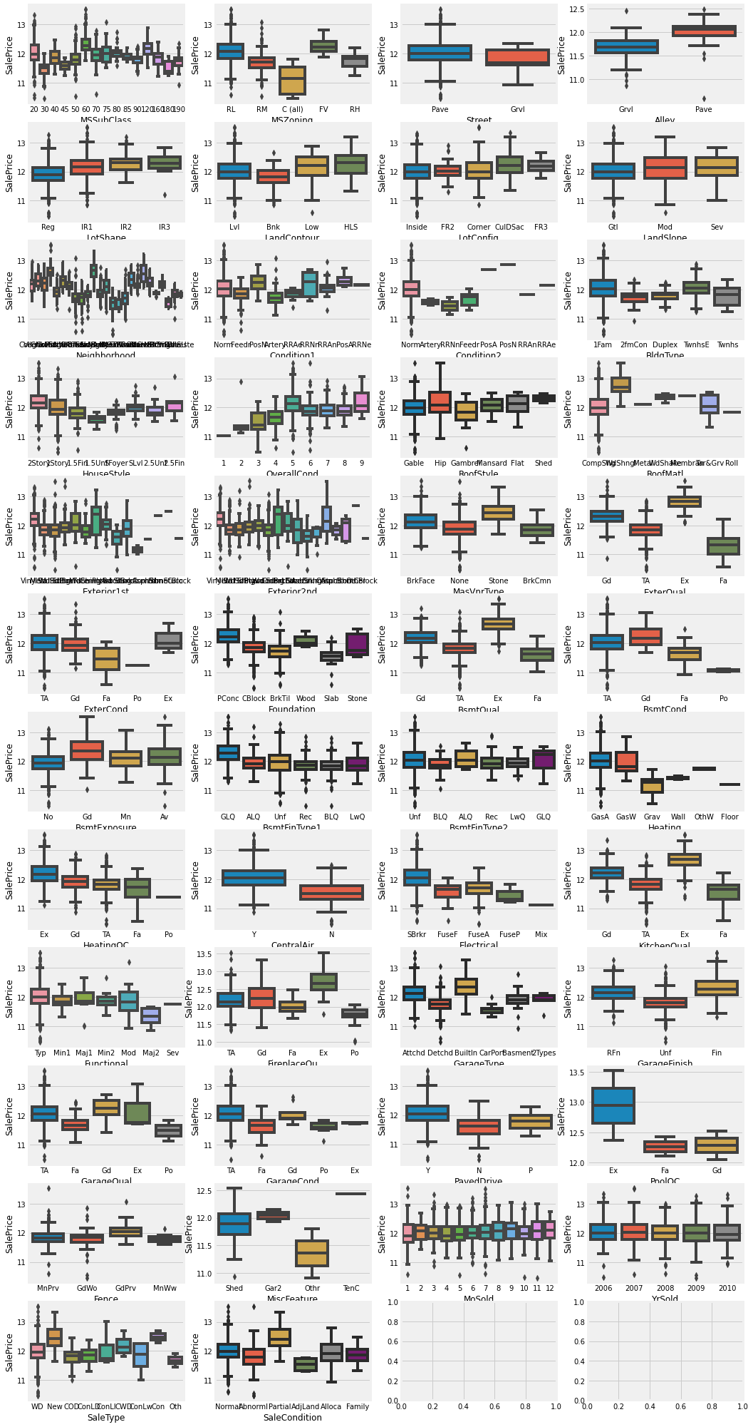
박스 플롯으로 비교하여 타겟변수에 영향을 많이 끼치는 변수들을 구분했다.
strong_obj = [ 'MSZoning', 'Neighborhood', 'Condition2', 'MasVnrType', 'ExterQual',
                'BsmtQual','CentralAir', 'Electrical', 'KitchenQual', 'SaleType']
for li in strong_obj:
sns.violinplot(x= li, y = target, data=train)
plt.show()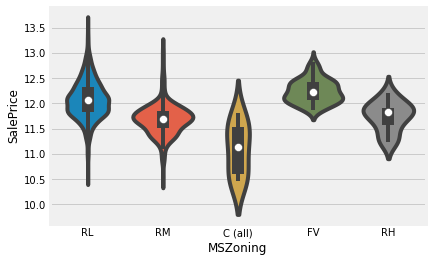
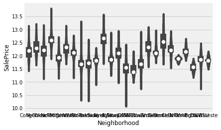
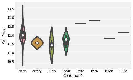
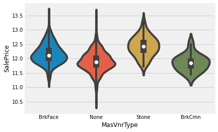
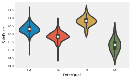
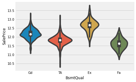
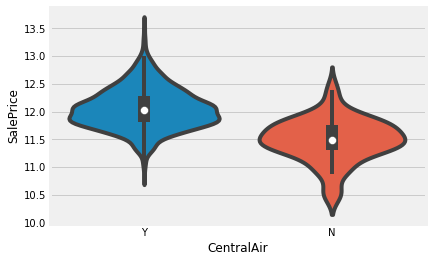
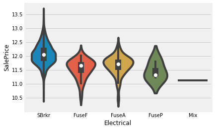
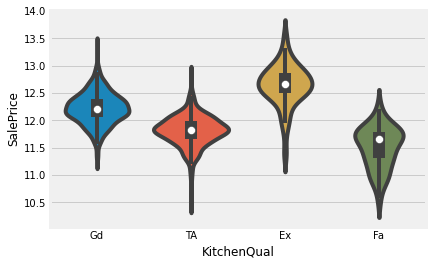
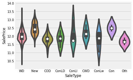
강한 변수들은 따로 Violine Plot 을 그려 확인했다.
numeric_features = df.dtypes[df.dtypes != "object"].indexfrom scipy.stats import skew
skewness = df[numeric_features].apply(lambda x: skew(x.dropna())).sort_values(ascending=False)왜도를 확인해보자.
high_skewness = skewness[abs(skewness) > 0.5]
skew_feat = high_skewness.index
print(high_skewness)
print(skew_feat)
MiscVal 21.919304
PoolArea 17.664161
haspool 15.473229
LotArea 13.167323
LowQualFinSF 12.067635
3SsnPorch 11.356127
LandSlope 4.987862
KitchenAbvGr 4.293726
BsmtFinSF2 4.169936
EnclosedPorch 4.021021
ScreenPorch 3.949857
BsmtHalfBath 3.923598
MasVnrArea 2.623822
OpenPorchSF 2.528620
WoodDeckSF 1.849679
Total_porch_sf 1.382622
Total_sqr_footage 1.248461
1stFlrSF 1.215511
LotFrontage 1.110062
GrLivArea 1.056757
BsmtFinSF1 0.983212
TotalSF 0.973652
BsmtUnfSF 0.914001
2ndFlrSF 0.852375
TotRmsAbvGrd 0.751009
Fireplaces 0.728641
HalfBath 0.693902
BsmtFullBath 0.625540
TotalBsmtSF 0.585973
OverallCond 0.563377
YearBuilt -0.594996
GarageFinish -0.611502
LotShape -0.618849
MoSold -0.646032
Alley -0.650364
BsmtExposure -1.118724
KitchenQual -1.451873
ExterQual -1.802942
Fence -1.988134
ExterCond -2.496596
BsmtCond -2.856010
PavedDrive -2.972363
BsmtFinType2 -3.052455
GarageQual -3.067326
CentralAir -3.451678
GarageCond -3.588285
GarageYrBlt -3.898299
hasgarage -3.933043
Functional -4.047595
hasbsmt -5.818135
Street -16.169674
PoolQC -21.188293
dtype: float64
Index(['MiscVal', 'PoolArea', 'haspool', 'LotArea', 'LowQualFinSF',
'3SsnPorch', 'LandSlope', 'KitchenAbvGr', 'BsmtFinSF2', 'EnclosedPorch',
'ScreenPorch', 'BsmtHalfBath', 'MasVnrArea', 'OpenPorchSF',
'WoodDeckSF', 'Total_porch_sf', 'Total_sqr_footage', '1stFlrSF',
'LotFrontage', 'GrLivArea', 'BsmtFinSF1', 'TotalSF', 'BsmtUnfSF',
'2ndFlrSF', 'TotRmsAbvGrd', 'Fireplaces', 'HalfBath', 'BsmtFullBath',
'TotalBsmtSF', 'OverallCond', 'YearBuilt', 'GarageFinish', 'LotShape',
'MoSold', 'Alley', 'BsmtExposure', 'KitchenQual', 'ExterQual', 'Fence',
'ExterCond', 'BsmtCond', 'PavedDrive', 'BsmtFinType2', 'GarageQual',
'CentralAir', 'GarageCond', 'GarageYrBlt', 'hasgarage', 'Functional',
'hasbsmt', 'Street', 'PoolQC'],
dtype='object')왜도가 0.5 이상인 칼럼은 따로 분류했다.
다 정규화시켜버릴 것이다.
df[['MiscVal', 'PoolArea', 'haspool', 'LotArea', 'LowQualFinSF',
       '3SsnPorch', 'LandSlope', 'KitchenAbvGr', 'BsmtFinSF2', 'EnclosedPorch',
       'ScreenPorch', 'BsmtHalfBath', 'MasVnrArea', 'OpenPorchSF',
       'WoodDeckSF', 'Total_porch_sf', '1stFlrSF', 'Total_sqr_footage',
       'LotFrontage', 'GrLivArea', 'TotalSF', 'BsmtFinSF1', 'BsmtUnfSF',
       '2ndFlrSF', 'TotRmsAbvGrd', 'Fireplaces', 'HalfBath', 'TotalBsmtSF',
       'BsmtFullBath', 'OverallCond', 'YearBuilt', 'GarageFinish', 'LotShape',
       'MoSold', 'Alley', 'BsmtExposure', 'KitchenQual', 'ExterQual', 'Fence',
       'ExterCond', 'BsmtCond', 'PavedDrive', 'BsmtFinType2', 'GarageQual',
       'CentralAir', 'GarageCond', 'GarageYrBlt', 'hasgarage', 'Functional',
       'hasbsmt', 'Street', 'PoolQC']].head(3)
다 박스콕스 시켜버릴 것이다.
from scipy.special import boxcox1p
lam = 0.15
for feat in skew_feat:
    df[feat] = boxcox1p(df[feat], lam)
df[['MiscVal', 'PoolArea', 'haspool', 'LotArea', 'LowQualFinSF',
'3SsnPorch', 'LandSlope', 'KitchenAbvGr', 'BsmtFinSF2', 'EnclosedPorch',
'ScreenPorch', 'BsmtHalfBath', 'MasVnrArea', 'OpenPorchSF',
'WoodDeckSF', 'Total_porch_sf', '1stFlrSF', 'Total_sqr_footage',
'LotFrontage', 'GrLivArea', 'TotalSF', 'BsmtFinSF1', 'BsmtUnfSF',
'2ndFlrSF', 'TotRmsAbvGrd', 'Fireplaces', 'HalfBath', 'TotalBsmtSF',
'BsmtFullBath', 'OverallCond', 'YearBuilt', 'GarageFinish', 'LotShape',
'MoSold', 'Alley', 'BsmtExposure', 'KitchenQual', 'ExterQual', 'Fence',
'ExterCond', 'BsmtCond', 'PavedDrive', 'BsmtFinType2', 'GarageQual',
'CentralAir', 'GarageCond', 'GarageYrBlt', 'hasgarage', 'Functional',
'hasbsmt', 'Street', 'PoolQC']].head(3)
정규화되었다.
레이블인코딩을 하지 않은 변수들에 대해서는 따로 get_dummies 를 사용하여 더미변수를 만들어주었다.
df = pd.get_dummies(df)
print(df.shape)
(2909, 230)
많기도 하다
# 중요변수 확인
new_train = df[:train.shape[0]]
new_test = df[train.shape[0]:]
new_train = pd.concat([new_train,target], axis=1, sort=False)corr_new_train = new_train.corr()
plt.figure(figsize=(5,15))
sns.heatmap(corr_new_train[['SalePrice']].sort_values(by=['SalePrice'],
ascending=False).head(30),annot=True)
상관성이 큰 변수들을 시각화해서 나타냈다.
col_corr_dict = corr_new_train['SalePrice'].sort_values(ascending=False).to_dict()best_columns=[]
for key,value in col_corr_dict.items():
if ((value>=0.33) & (value<0.9)) | (value<=-0.325):
best_columns.append(key)
print(len(best_columns))39상관계수가 약 0.33 보다 큰. 상관계수가 큰 변수들을 뽑았더니 39개가 나왔다.
new_train = new_train.drop(['SalePrice'], axis=1)
new_train = new_train.drop(['Id'], axis=1)
new_test = new_test.drop(['Id'], axis=1)
train 데이터에서 필요없는 목적변수와 ID 값을 test에서도 제거해주었다.
final_train = new_train[best_columns]
final_test = new_test[best_columns]
final_num = list(final_train.columns)
이제 최종 변수들을 모두 final_ 변수들에 넣어주었다.
변수.최종최종최종
row = 19
col = 2

fig, axs = plt.subplots(row,col, figsize = (20,60))
fig.subplots_adjust(hspace=0.8)

for r in range(0,row):
    for c in range(0,col):
        i = r*col + c
        if i < len(best_columns):
            sns.regplot(final_train[final_num[i]],target,fit_reg=True,marker='o', ax = axs[r][c])
마지막으로 regplot 한 번 더 확인하기.
이상치를 더 제거하면ㄴ 모델 성능이 더 높아질 수 있을것이라고 생각이 든다.
변수가 많아서 처리할 게 많아 포스팅이 길다 ..
모델링 과정은 다음에 ..
도움받은 분들
말이 도움이지 그대로 따라한 것이나 다름이 없음.
저는 이 분들의 것을 합쳐서 필사하며 공부했습니다 !
[Kaggle] 보스턴 주택 가격 예측(House Prices: Advanced Regression Techniques)
Intro캐글의 고전적인 문제이며 머신러닝을 공부하는 사람이라면 누구나 한번쯤 다뤄봤을 Boston house price Dataset을 통해 regression하는 과정을 소개하려 한다. 정식 competition 명칭은 'House Prices: Advanced
velog.io
https://minding-deep-learning.tistory.com/16
[Kaggle] House Prices Prediction : 보스턴 주택가격 예측 - 1. EDA & Feature Engineering
[파이썬 라이브러리를 활용한 머신러닝] 책을 공부하던 때 처음 접해보았던 머신러닝 회귀 문제의 대표문제, Kaggle의 House Prices 예측 데이터셋을 다시 한번 살펴보는 시간을 가졌다. 데이터셋은 K
minding-deep-learning.tistory.com
https://hong-yp-ml-records.tistory.com/2
[House Prices] Tutorial For Korean Beginners - 캐글 집값 예측 part 1
House Prices Predict 아이오와 주 에임스에 있는 주거용 주택의 모든 측면을 설명하는 79 개의 변수로 주택의 판매가격을 예측하는 Competition입니다. Introduction 본 커널은 다수의 고수분들이 올려주신
hong-yp-ml-records.tistory.com
https://www.kaggle.com/code/munmun2004/house-prices-for-begginers/notebook
[한글커널][House Prices]보스턴 집값 예측 for Begginers
Explore and run machine learning code with Kaggle Notebooks | Using data from House Prices - Advanced Regression Techniques
www.kaggle.com


